A Bayesian foundation for individual learning under uncertainty
- 1 Laboratory for Social and Neural Systems Research, Department of Economics, University of Zurich, Zurich, Switzerland
- 2 Institute for Biomedical Engineering, Eidgenössische Technische Hochschule Zurich, Zurich, Switzerland
- 3 Wellcome Trust Centre for Neuroimaging, Institute of Neurology, University College London, London, UK
Computational learning models are critical for understanding mechanisms of adaptive behavior. However, the two major current frameworks, reinforcement learning (RL) and Bayesian learning, both have certain limitations. For example, many Bayesian models are agnostic of inter-individual variability and involve complicated integrals, making online learning difficult. Here, we introduce a generic hierarchical Bayesian framework for individual learning under multiple forms of uncertainty (e.g., environmental volatility and perceptual uncertainty). The model assumes Gaussian random walks of states at all but the first level, with the step size determined by the next highest level. The coupling between levels is controlled by parameters that shape the influence of uncertainty on learning in a subject-specific fashion. Using variational Bayes under a mean-field approximation and a novel approximation to the posterior energy function, we derive trial-by-trial update equations which (i) are analytical and extremely efficient, enabling real-time learning, (ii) have a natural interpretation in terms of RL, and (iii) contain parameters representing processes which play a key role in current theories of learning, e.g., precision-weighting of prediction error. These parameters allow for the expression of individual differences in learning and may relate to specific neuromodulatory mechanisms in the brain. Our model is very general: it can deal with both discrete and continuous states and equally accounts for deterministic and probabilistic relations between environmental events and perceptual states (i.e., situations with and without perceptual uncertainty). These properties are illustrated by simulations and analyses of empirical time series. Overall, our framework provides a novel foundation for understanding normal and pathological learning that contextualizes RL within a generic Bayesian scheme and thus connects it to principles of optimality from probability theory.
Introduction
Learning can be understood as the process of updating an agent’s beliefs about the world by integrating new and old information. This enables the agent to exploit past experience and improve predictions about the future; e.g., the consequences of chosen actions. Understanding how biological agents, such as humans or animals, learn requires a specification of both the computational principles and their neurophysiological implementation in the brain. This can be approached in a bottom-up fashion, building a neuronal circuit from neurons and synapses and studying what forms of learning are supported by the ensuing neuronal architecture. Alternatively, one can choose a top-down approach, using generic computational principles to construct generative models of learning and use these to infer on underlying mechanisms (e.g., Daunizeau et al., 2010a). The latter approach is the one that we pursue in this paper.
The laws of inductive inference, prescribing an optimal way to learn from new information, have long been known (Laplace, 1774, 1812). They have a unique mathematical form, i.e., it has been proven that there is no alternative formulation of inductive reasoning that does not violate either consistency or common sense (Cox, 1946). Inductive reasoning is also known as Bayesian learning because the requisite updating of conditional probabilities is described by Bayes’ theorem. Since a Bayesian learner processes information optimally, it should have an evolutionary advantage over other types of agents, and one might therefore expect the human brain to have evolved such that it implements an ideal Bayesian learner (Geisler and Diehl, 2002). Indeed, there is substantial evidence from studies on various domains of learning and perception that human behavior is better described by Bayesian models than by other theories (e.g., Kording and Wolpert, 2004; Bresciani et al., 2006; Yuille and Kersten, 2006; Behrens et al., 2007; Xu and Tenenbaum, 2007; Orbán et al., 2008; den Ouden et al., 2010). However, there remain at least three serious difficulties with the hypothesis that humans act as ideal Bayesian learners. The first problem is that in all but the simplest cases, the application of Bayes’ theorem involves complicated integrals that require burdensome and time-consuming numerical calculations. This makes online learning a challenging task for Bayesian models, and any evolutionary advantage conferred by optimal learning might be outweighed by these computational costs. A second and associated problem is how ideal Bayesian learning, with its requirement to evaluate high-dimensional integrals, would be implemented neuronally (cf. Yang and Shadlen, 2007; Beck et al., 2008; Deneve, 2008). The third difficulty is that Bayesian learning constitutes a normative framework that prescribes how information should be dealt with. In reality, though, even when endowed with equal prior knowledge, not all agents process new information alike. Instead, even under carefully controlled conditions, animals and humans display considerable inter-individual variability in learning (e.g., Gluck et al., 2002; Daunizeau et al., 2010b). Despite previous attempts of Bayesian models to deal with individual variability (e.g., Steyvers et al., 2009; Nassar et al., 2010), the failure of orthodox Bayesian learning theory to account for these individual differences remains a key problem for understanding (mal)adaptive behavior of humans. Formal and mechanistic characterizations of this inter-subject variability are needed to comprehend fundamental aspects of brain function and disease. For example, individual differences in learning may result from inter-individual variability in basic physiological mechanisms, such as the neuromodulatory regulation of synaptic plasticity (Thiel et al., 1998), and such differences may explain the heterogeneous nature of psychiatric diseases (Stephan et al., 2009).
These difficulties have been avoided by descriptive approaches to learning, which are not grounded in probability theory, notably some forms of reinforcement learning (RL), where agents learn the “value” of different stimuli and actions (Sutton and Barto, 1998; Dayan and Niv, 2008). While RL is a wide field encompassing a variety of schemes, perhaps the most prototypical and widely used model is that by Rescorla and Wagner (1972). In this description, predictions of value are updated in relation to the current prediction error, weighted by a learning rate (which may differ across individuals and contexts). The great advantage of this scheme is its conceptual simplicity and computational efficiency. It has been applied empirically to various learning tasks (Sutton and Barto, 1998) and has played a major role in attempts to explain electrophysiological and functional magnetic resonance imaging (fMRI) measures of brain activity during reward learning (e.g., Schultz et al., 1997; Montague et al., 2004; O’Doherty et al., 2004; Daw et al., 2006). Furthermore, its non-normative descriptive nature allows for modeling aberrant modes of learning, such as in schizophrenia or depression (Smith et al., 2006; Murray et al., 2007; Frank, 2008; Dayan and Huys, 2009). Similarly, it has found widespread use in modeling the effects of neuromodulatory transmitters, such as dopamine, on learning (e.g., Yu and Dayan, 2005; Pessiglione et al., 2006; Doya, 2008).
Despite these advantages, RL also suffers from major limitations. On the theoretical side, it is a heuristic approach that does not follow from the principles of probability theory. In practical terms, it often performs badly in real-world situations where environmental states and the outcomes of actions are not known to the agent, but must also be inferred or learned. These practical limitations have led some authors to argue that Bayesian principles and “structure learning” are essential in improving RL approaches (Gershman and Niv, 2010). In this article, we introduce a novel model of Bayesian learning that overcomes the three limitations of ideal Bayesian learning discussed above (i.e., computational complexity, questionable biological implementation, and failure to account for individual differences) and that connects Bayesian learning to RL schemes.
Any Bayesian learning scheme relies upon the definition of a so-called “generative model,” i.e., a set of probabilistic assumptions about how sensory signals are generated. The generative model we propose is inspired by the seminal work of Behrens et al. (2007) and comprises a hierarchy of states that evolve in time as Gaussian random walks, with each walk’s step size determined by the next highest level of the hierarchy. This model can be inverted (fitted) by an agent using a mean-field approximation and a novel approximation to the conditional probabilities over unknown quantities that replaces the conventional Laplace approximation. This enables us to derive closed-form update equations for the posterior expectations of all hidden states governing contingencies in the environment. This results in extremely efficient computations that allow for real-time learning. The form of these update equations is similar to those of Rescorla–Wagner learning, providing a Bayesian analogon to RL theory. Finally, by introducing parameters that determine the nature of the coupling between the levels of the hierarchical model, the optimality of an update is made conditional upon parameter values that may vary from agent to agent. These parameters encode prior beliefs about higher-order structure in the environment and enable the model to account for inter-individual (and inter-temporal intra-individual) differences in learning. In other words, the model is capable of describing behavior that is subjectively optimal (in relation to the agent’s prior beliefs) but objectively maladaptive. Importantly, the model parameters that determine the nature of learning may relate to specific physiological processes, such as the neuromodulation of synaptic plasticity. For example, it has been hypothesized that dopamine, which regulates plasticity of glutamatergic synapses (Gu, 2002), may encode the precision of prediction errors (Friston, 2009). In our model, this precision-weighting of prediction errors is determined by the model’s parameters (cf. Figure 4). Ultimately, our approach may therefore be useful for model-based inference on subject-specific computational and physiological mechanisms of learning, with potential clinical applications for diagnostic classifications of psychiatric spectrum disorders (Stephan et al., 2009).
To prevent any false expectations, we would like to point out that this paper is of a purely theoretical nature. Its purpose is to introduce the theoretical foundations and derivation of our model in detail and convey an understanding of the phenomena it can capture. Owing to length restrictions and to maintain clarity and focus, several important aspects cannot be addressed in this paper. For example, it is beyond the scope of this initial theory paper to investigate the numerical exactness of our variational inversion scheme, present applications of model selection, or present evidence that our model provides for more powerful inference on learning mechanisms from empirical data than other approaches. These topics will be addressed in forthcoming papers by our group.
This paper is structured as follows: First, we derive the general structure of the model, level by level, and consider both its exact and variational inversion. We then present analytical update equations for each level of the model that derive from our variational approach and a quadratic approximation to the variational energies. Following a structural interpretation of the model’s update equations in terms of RL, we present simulations in which we demonstrate the model’s behavior under different parameter values. Finally, we illustrate the generality of our model by demonstrating that it can equally deal with (i) discrete and continuous environmental states, and (ii) deterministic and probabilistic relations between environmental and perceptual states (i.e., situations with and without perceptual uncertainty).
Theory
The Generative Model Under Minimal Assumptions
An overview of our generative model is given by Figures 1 and 2. To model learning in general terms, we imagine an agent who receives a sequence of sensory inputs u(1), u(2),…,u(n). Given a generative model of how the agent’s environment generates these inputs, probability theory tells us how the agent can make optimal use of the inputs u(1),…,u(k−1) and any further “prior” information to predict the next input u(k). The generative model we introduce here is an extension of the model proposed by Daunizeau et al. (2010b) and also draws inspiration from the work by Behrens et al. (2007). Our model is very general: it can deal with states and inputs that are discrete or continuous and uni- or multivariate, and it equally accounts for deterministic and probabilistic relationships between environmental events and perceptual states (i.e., situations with and without perceptual uncertainty). However, to keep the mathematical derivation as simple as possible, we initially deal with an environment where the sensory input u(k) ∈ {0, 1} on trial k is of a binary form; note that this can be readily extended to much more complex environments and input structures. In fact, at a later stage we will also deal with stochastic mappings (i.e., perceptual uncertainty; cf. Eq. 45) and continuous (real-valued) inputs and states (cf. Eq. 48).
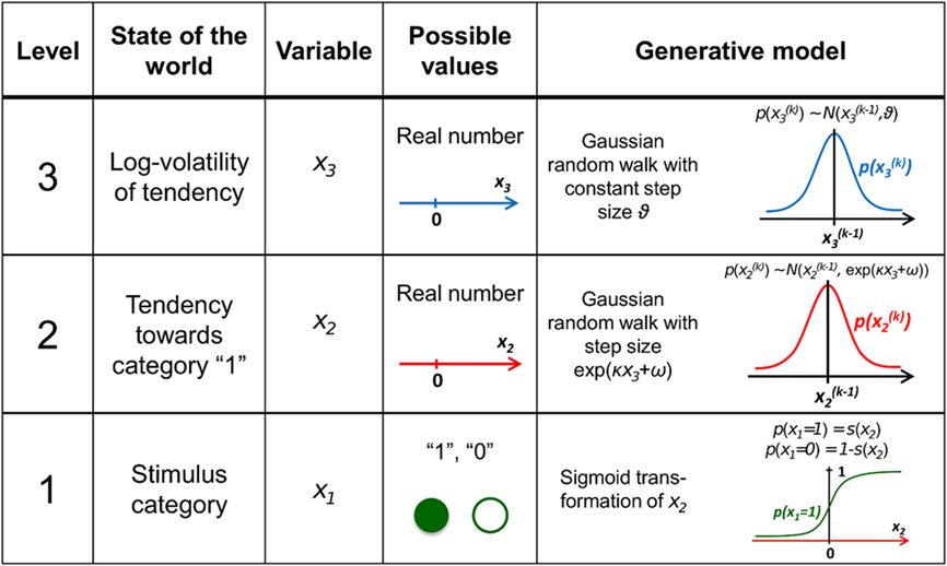
Figure 1. Overview of the hierarchical generative model. The probability at each level is determined by the variables and parameters at the next highest level. Note that further levels can be added on top of the third. These levels relate to each other by determining the step size (volatility or variance) of a random walk. The topmost step size is a constant parameter ϑ. At the first level, x1 determines the probability of the input u.
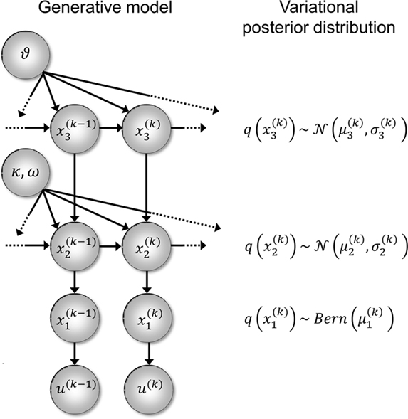
Figure 2. Generative model and posterior distributions on hidden states. Left: schematic representation of the generative model as a Bayesian network.  are hidden states of the environment at time point k. They generate u(k), the input at time point k, and depend on their immediately preceding values
  ,
,  and the parameters ϑ, ω, κ. Right: the minimal parametric description q(x) of the posteriors at each level. The distribution parameters μ (posterior expectation) and σ (posterior variance) can be found by approximating the minimal parametric posteriors to the mean-field marginal posteriors. For multidimensional states x, μ is a vector and σ a covariance matrix.
For simplicity, imagine a situation where the agent is only interested in a single (binary) state of its environment; e.g., whether it is light or dark. In our model, the environmental state x1 at time k, denoted by  causes input u(k). Here,
  could represent the on/off state of a light switch and u the sensation of light or darkness. (For simplicity, we shall often omit the time index k). In the following, we assume the following form for the likelihood model:

In other words: u = x1 for both x1 = 1 and x1 = 0 (and vice versa). This means that knowing state x1 allows for an accurate prediction of input u: when the switch is on, it is light; when it is off, it is dark. The deterministic nature of this relation does not affect the generality of our argument and will later be replaced by a stochastic mapping when dealing with perceptual uncertainty below.
Since x1 is binary, its probability distribution can be described by a single real number, the state x2 at the next level of the hierarchy. We then map x2 to the probability of x1 such that x2 = 0 means that x1 = 0 and x1 = 1 are equally probable. For x2 → ∞ the probability for x1 = 1 and x1 = 0 should approach 1 and 0, respectively. Conversely, for x2 → ∝ the probabilities for x1 = 1 and x1 = 0 should approach 0 and 1, respectively. This can be achieved with the following empirical (conditional) prior density:

where s(·) is a sigmoid (softmax) function:
Put simply, x2 is an unbounded real parameter of the probability that x1 = 1. In our light/dark example, one might interpret x2 as the tendency of the light to be on.
For the sake of generality, we make no assumptions about the probability of x2 except that it may change with time as a Gaussian random walk. This means that the value of x2 at time k will be normally distributed around its value at the previous time point, 

Importantly, the dispersion of the random walk (i.e., the variance exp(κx3 + ω) of the conditional probability) is determined by the parameters κ and ω (which may differ across agents) as well as by the state x3. Here, this state determines the log-volatility of the environment (cf. Behrens et al., 2007, 2008). In other words, the tendency x2 of the light switch to be on performs a Gaussian random walk with volatility exp(κx3 + ω). Introducing ω allows for a volatility that scales independently of the state x3. Everything applying to x2 now equally applies to x3, such that we could add as many levels as we please. Here, we stop at the fourth level, and set the volatility of x3 to ϑ, a constant parameter (which may again differ across agents):

Given full priors on the parameters, i.e., p(κ, ω, ϑ), we can now write the full generative model
Given priors on the initial state  the generative model is defined for all times k by recursion to k = 1. Inverting this model corresponds to optimizing the posterior densities over the unknown (hidden) states x = {x1, x2, x3} and parameters χ = {κ, ω, ϑ}. This corresponds to perceptual inference and learning, respectively. In the next section, we consider the nature of this inversion or optimization.
Exact Inversion
It is instructive to consider the factorization of the generative density
In this form, the Markovian structure of the model becomes apparent: the joint probability of the input and the states at time k depends only on the states at the immediately preceding time k − 1. It is the probability distribution of these states that contains the information conveyed by previous inputs  i.e.:
i.e.:

By integrating out  and
and  we obtain the following compact form of the generative model at time k:
Once u(k) is observed, we can plug it into this expression and obtain

This is the quantity of interest to us, because it describes the posterior probability of the time-dependent states, x(k) (and time-independent parameters, χ), in the agent’s environment. This is what the agent infers (and learns), given the history of previous inputs. Computing this probability is called model inversion: unlike the likelihood p(u(k)|x(k), χ, u(1…k - 1)) the posterior does not predict data (u(k)) from hidden states and parameters but predicts states and parameters from data.
In the framework we introduce here, we model the individual variability between agents by putting delta-function priors on the parameters:
where χa are the fixed parameter values that characterize a particular agent at a particular time (e.g., during the experimental session). This corresponds to the common distinction between states (as variables that change quickly) and parameters (as variables that change slowly or not at all). In other words, we assume that the timescale at which parameter estimates change is much larger than the one on which state estimates change, and also larger than the periods during which we observe agents in a single experiment. This is not a strong assumption, given that the model has multiple hierarchical levels of states that give the agent the required flexibility to adapt its beliefs to a changing environment. In effect, this approach gives us a family of Bayesian learners whose (slowly changing) individuality is captured by their priors on the parameters. For other examples where subjects’ beliefs about the nature of their environment were modeled as priors on parameters, see Daunizeau et al. (2010b) and Steyvers et al. (2009).
In principle, model inversion can proceed in an online fashion: By (numerical) marginalization, we can obtain the (marginal) posteriors  and
and  this is the approach adopted by Behrens et al. (2007), allowing one to compute p(u(k+1), x(k+1), χ|u(1…k)) according to Eq. 6, and subsequently p(u(k+1), χ|u(1…k+1)) once u(k+1) becomes known, and so on. Unfortunately, this (exact) inversion involves many complicated (non-analytical) integrals for every new input, rendering exact Bayesian inversion unsuitable for real-time learning in a biological setting. If the brain uses a Bayesian scheme, it is likely that it relies on some sufficiently accurate, but fast, approximation to Eq. 9: this is approximate Bayesian inference. As described in the next section, a generic and efficient approach is to employ a mean-field approximation within a variational scheme. This furnishes an efficient solution with biological plausibility and interpretability.
Variational Inversion
Variational Bayesian (VB) inversion determines the posterior distributions p(x(k), χ|u(1…k)) by maximizing the log-model evidence. The log-evidence corresponds to the negative surprise about the data, given a model, and is approximated by a lower bound, the negative free energy. Detailed treatments of the general principles of the VB procedure can be found in numerous papers (e.g., Beal, 2003; Friston and Stephan, 2007). The approximations inherent in VB enable a computationally efficient inversion scheme with closed-form single-step probability updates from trial to trial. In particular, VB can incorporate the so-called mean-field approximation which turns the joint posterior distribution into the product of approximate marginal posterior distributions:
Based on this assumption, the variational maximization of the negative free energy is implemented in a series of variational updates for each level i of the model separately. The second line in Eq. 11 represents the mean-field assumption (factorization of the posterior), while the third line reflects the fact that we assume a fixed form q(·) for the approximate marginals  We make minimal assumptions about the form of the approximate posteriors by following the maximum entropy principle: given knowledge of, or assumptions about, constraints on a distribution, the least arbitrary choice of distribution is the one that maximizes entropy (Jaynes, 1957). To keep the description of the posteriors simple and biologically plausible, we take them to be characterized only by their first two moments; i.e., by their mean and variance. At the first level, we have a binary state x1 with a mean μ1 = p(x1 = 1). Under this constraint, the maximum entropy distribution is the Bernoulli distribution with parameter μ1 (where the variance μ1(1 − μ1) is a function of the mean):
At the second and third level, the maximum entropy distribution of the unbounded real variables x2 and x3, given their means and variances, is Gaussian. Note that the choice of a Gaussian distribution for the approximate posteriors is not due simply to computational expediency (or the law of large numbers) but follows from the fact that, given the assumption that the posterior is encoded by its first two moments, the maximum entropy principle prescribes a Gaussian distribution. Labeling the means μ2, μ3 and the variances σ2, σ3, we obtain


Now that we have approximate posteriors q that we treat as known for all but the ith level, the next step is to determine the variational posterior  for this level i. Variational calculus shows that given q(xj) (j ∈ {1, 2, 3} and j ≠ i), the approximate posterior
  under the mean-field approximation is proportional to the exponential of the variational energy I(xi) (Beal, 2003):
 is a normalization constant that ensures that the integral (or sum, in the discrete case) of
  over x equals unity. Under our generative model, the variational energy is
where x\i denotes all xj with j ≠ i and X\i is the direct product of the ranges (or values in the discrete case) of the xj contained in x\i. The integral over discrete values is again a sum. In what follows, we take this general theory and unpack it using the generative model for sequential learning above. Our special focus here will be on the form of the variational updates that underlie inference and learning and how they may be implemented in the brain.
Results
The Variational Energies
To compute  , we need
  and therefore the sufficient statistics λ\i = {μ\i,σ\i} for the posteriors at all but the ith level. One could try to extract them from
  but that would constitute a circular problem. We avoid this by exploiting the hierarchical form of the model: for the first level, we use the sufficient statistics of the higher levels from the previous time point k − 1, since information about input u(k) cannot yet have reached those levels. From there we proceed upward through the hierarchy of levels, always using the updated parameters
  for levels lower than the current level and pre-update values
  for higher levels. Extending the approach suggested by Daunizeau et al. (2010b), and using power series approximations where necessary, the variational energy integrals can then be calculated for all xi, giving
Substituting these variational energies into Eq. 15, we obtain the posterior distribution of x under the mean-field approximation.
According to Eqs 15 and 17–19,  depends on u(k),

 and χ. In the next section, we show that it is possible to derive simple closed-form Markovian update equations of the form

Update equations of this form allow the agent to update its approximate posteriors over  very efficiently and thus optimize its beliefs about the environment in real time. We now consider the detailed form of these equations and how they relate to classical heuristics from RL.
The Update Equations
At the first level of the model, it is simple to determine q(x1) since  is a Bernoulli distribution with parameter

and therefore already has the form required of q(x1) by Eq. 12. We can thus take  and have in Eq. 21 an update rule of the form of Eq. 20.
At the second level,  does not have the form required of q(x2) by Eq. 13 since it is only approximately Gaussian. It is proportional to the exponential of I(x2) and would only be Gaussian if I(x2) were quadratic. The problem of finding a Gaussian approximation
  can therefore be reformulated as finding a quadratic approximation to I(x2). The obvious way to achieve this is to expand I(x2) in powers of x2 up to second order. The choice of expansion point, however, is not trivial. One possible choice is the mode or maximum of I(x2), resulting in the frequently used Laplace approximation (Friston et al., 2007). This has the disadvantage that the maximum of I(x2) is unknown and has to be found by numerical optimization methods, precluding a single-step analytical update rule of the form of Eq. 20 (this is no problem in a continuous time setting, where the mode of the variational energy can be updated continuously (cf. Friston, 2008)). However, for the discrete updates we seek, one can use the expectation
  as the expansion point for time k, when the agent receives input u(k) and the expectation of
  is
is  In terms of computational and mnemonic costs, this is the most economical choice since this value is known. Moreover, it yields analytical update equations which (i) bear structural resemblance to those used by RL models (see Structural Interpretation of the Update Equations) and (ii) can be computed very efficiently in a single step:

where, for clarity, we have used the definitions


formulated in terms of precisions (inverse variances) 

 the variance update (Eq. 22) takes the simple form
in the context of the update equations, we use the hat notation to indicate “referring to prediction.” While the  are the predictions before seeing the input u(k), the
  and
and  are the variances (i.e., uncertainties) and precisions of these predictions (see Structural Interpretation of the Update Equations).
The approach that produces these update equations is conceptually similar to a Gauss–Newton ascent on the variational energy that would, by iteration, produce the Laplace approximation (cf. Figure 3). The same approach can be taken at the third level, where we also have a Gaussian approximate posterior:
with  and
and
The derivation of these update equations, based on this novel quadratic approximation to I(x2) and I(x3), is described in detail in the next section, and Figure 3 provides a graphical illustration of the ensuing procedure. The meaning of the terms that appear in the update equations and the overall structure of the updates will be discussed in detail in the Section “Structural Interpretation of the Update Equations.”
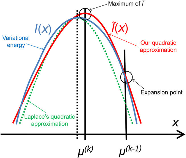
Figure 3. Quadratic approximation to the variational energy. Approximating the variational energy I(x) (blue) by a quadratic function leads (by exponentiation) to a Gaussian posterior. To find our approximation Ĩ(x) (red), we expand I(x) to second order at the preceding posterior expectation μ(k−1). The argmax of Ĩ(x) is then the new posterior expectation μ(k). This generally leads to a different result from the Laplace approximation (dashed), but there is a priori no reason to regard either approximation as more exact than the other.
Quadratic Approximation to the Variational Energies
While knowing I(xi) (with i = 1, 2, 3) gives us the unconstrained posterior  given q(x\i), we still need to determine the constrained posterior q(xi) for all but the first levels, where
  Schematically, our approximation procedure can be pictured in the following way:
We denote by Ĩ the quadratic function obtained by expansion of I around  (see Figure 3 for a graphical summary). Its exponential has the Gaussian form required by Eqs 13 and 14 (where
  is a normalization constant):
This equation lets us find  and
and  Taking the logarithm on both sides and then differentiating twice with respect to
  gives
gives
where ∂2 denotes the second derivative, which is constant for a quadratic function. Because ∂2I and ∂2Ĩ agree at the expansion point  we may write
A somewhat different line of reasoning leads to  Since
Since  is the argument of the maximum (argmax) of q (and exponentiation preserves the argmax)
  has to be the argmax of Ĩ. Starting at any point
  the exact argmax of a quadratic function can be found in one step by Newton’s method:
If we choose  to be the expansion point
  we have agreement of I with Ĩ up to the second derivative at this point and may therefore write
Plugging I(x2) from Eq. 18 into Eqs 38 and 40 now yields the parameter update equations (Eqs 22 and 23) of the form Eq. 20 for the second level. For the third level (or indeed any higher level with an approximately Gaussian posterior distribution we may wish to include), the same procedure gives Eqs 29 and 30. Note that this method of obtaining closed-form Markovian parameter update equations can readily be applied to multidimensional xi’s with approximately multivariate Gaussian posteriors by reinterpreting ∂I as a gradient and 1/∂2I as the inverse of a Hessian in Eqs 38 and 40.
Structural Interpretation of the Update Equations
As we have seen, variational inversion of our model, using a new quadratic approximation to the variational energies, provides a set of simple trial-by-trial update rules for the sufficient statistics λi = {μi, σi} of the posterior distributions we seek. These update equations do not increase in complexity with trials, in contrast to exact Bayesian inversion, which requires analytically intractable integrations (cf. Eq. 9). In our approach, almost all the work is in deriving the update rules, not in doing the actual updates.
Crucially, the update equations for μ2 and μ3 have a form that is familiar from RL models such as Rescorla–Wagner learning (Figure 4). The general structure of RL models can be summarized as:

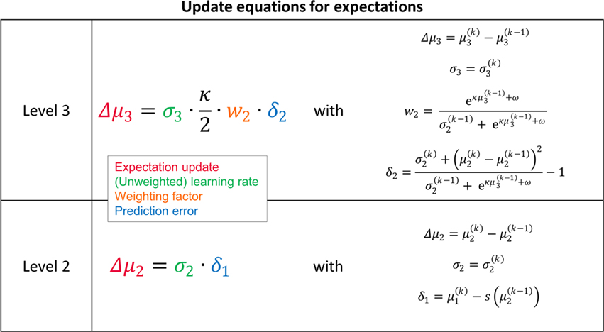
Figure 4. Interpretation of the variational update equations in terms of Rescorla–Wagner learning. The Rescorla–Wagner update is Δprediction = learning rate × prediction error. Our expectation update equations can be interpreted in these terms.
As we explain in detail below, this same structure appears in Eqs 23 and 30 – displayed here in their full forms:
The term  in Eq. 23 corresponds to the prediction error at the first level. This prediction error is the difference between the expectation
  of x1 having observed input u(k) and the prediction
  before receiving u(k); i.e., the softmax transformation of the expectation of x2 before seeing u(k). Furthermore,
  in Eq. 23 can be interpreted as the equivalent of a (time-varying) learning rate in RL models (cf. Preuschoff and Bossaerts, 2007). Since σ2 represents the width of x2’s posterior and thus the degree of our uncertainty about x2, it makes sense that updates in μ2 are proportional to this estimate of posterior uncertainty: the less confident the agent is about what it knows, the greater the influence of new information should be.
According to its update Eq. 22, μ2 always remains positive since it contains only positive terms. Crucially, σ2, through  depends on the log-volatility estimate μ3, from the third level of the model. For vanishing volatility, i.e.,
  σ2 can only decrease from trial to trial. This corresponds to the case in which the agent believes that x2 is fixed; the information from every trial then has the same weight and new information can only shrink σ2. On the other hand, even with
  σ2 has a lower bound: when σ2 approaches zero, the denominator of Eq. 22 approaches 1/σ2 from above, leading to ever smaller decreases in σ2. This means that after a long train of inputs, the agent still learns from new input, even when it infers that the environment is stable.
The precision formulation (cf. Eq. 28)
illustrates that three forms of uncertainty influence the posterior variance  the informational
  and the environmental
  uncertainty at the second level (see discussion in the next paragraph), and the uncertainty
  of the prediction at the first level. While environmental uncertainty at the second level thus decreases precision
  relative to its previous value
  predictive uncertainty at the first level counteracts that decrease, i.e., it keeps the learning rate
  smaller than it would otherwise be. This makes sense because prediction error should mean less when predictions are more uncertain.
The update rule (Eq. 30) for μ3 has a similar structure to that of μ2 (Eq. 23) and can also be interpreted in terms of RL. Although perhaps not obvious at first glance,  (Eq. 34) represents prediction error. It is positive if the updates at the second level (of μ2 and σ2) in response to input u(k) indicate that the agent was underestimating x3. Conversely, it is negative if the agent was overestimating x3. This can be seen by noting that the uncertainty about x2 has two sources: informational, i.e., the lack of knowledge about x2 (represented by σ2), and environmental, i.e., the volatility of the environment (represented by
  ). Before receiving input u(k) the total uncertainty is
  After receiving the input, the updated total uncertainty is
  where σ2 has been updated according to Eq. 22 and
  has been replaced by the squared update of μ2. If the total uncertainty is greater after seeing u(k), the fraction in
  is greater than one, and μ3 increases. Conversely, if seeing u(k) reduces total uncertainty, μ3 decreases. (Since x3 is on a logarithmic scale with respect to x2, the ratio and not the difference of quantities referring to x2 is relevant for the prediction error in x3). It is important to note that we did not construct the update equations with any of these properties in mind. It is simply a reflection of Bayes optimality that emerges on applying our variational update method.
The term corresponding to the learning rate of μ3 is
As at the second level, this is proportional to the variance σ3of the posterior. But here, the learning rate is also is proportional to the parameter κ and a weighting factor
 for prediction error. κ determines the form of the Gaussian random walk at the second level and couples the third level to the second (cf. Eqs 4 and 30);
  is a measure of the (environmental) volatility
  of x2 relative to its (informational) conditional uncertainty, σ2. It is bounded between 0 and 1 and approaches 0 as
  becomes negligibly small relative to σ2; conversely, it approaches 1 as σ2 becomes negligibly small relative to
  This means that lack of knowledge about x2 (i.e., conditional uncertainty σ2) suppresses updates of μ3 by reducing the learning rate, reflecting the fact that prediction errors in x2 are only informative if the agent is confident about its predictions of x2. As with the prediction error term, this weighting factor emerged from our variational approximation.
The precision update (Eq. 29) at third level also has an interpretable form. In addition to  and
and  we now also have the term
  (Eq. 33), which is the relative difference of environmental and informational uncertainty (i.e., relative to their sum). Note that it is a simple affine function of the weighting factor

As at the second level, the precision update is the sum of the precision  of the prediction, reflecting the informational and environmental uncertainty at the third level, and the term
Proportionality to κ2 reflects the fact that stronger coupling between the second and third levels leads to higher posterior precision (i.e., less posterior uncertainty) at the third level, while proportionality to w2 depresses precision at the third level when informational uncertainty at the second level is high relative to environmental uncertainty; the latter also applies to the first summand in the brackets. The second summand r2δ2 means that, when the agent regards environmental uncertainty at the second level as relatively high (r2 > 0), volatility is held back from rising further if δ2 > 0 by way of a decrease in the learning rate (which is proportional to the inverse precision), but conversely pushed to fall if δ2 < 0. If, however, environmental uncertainty is relatively low (r2 < 0), the opposite applies: positive volatility prediction errors increase the learning rate, allowing the environmental uncertainty to rise more easily, while negative prediction errors decrease the learning rate. The term r2δ2 thus exerts a stabilizing influence on the estimate of μ3.
This automatic integration of all the information relevant to a situation is typical of Bayesian methods and brings to mind a remark made by Jaynes (2003, p. 517) in a different context: “This is still another example where Bayes’ theorem detects a genuinely complicated situation and automatically corrects for it, but in such a slick, efficient way that one is [at first, we would say] unaware of what is happening.” In the next section we use simulations to illustrate the nature of this inference and demonstrate some of its more important properties.
Simulations
Here, we present several simulations to illustrate the behavior of the update equations under different values of the parameters ϑ, ω, and κ. Figure 5 depicts a “reference” scenario, which will serve as the basis for subsequent variations. Figures 6–8 display the effects of selectively changing one of the parameters ϑ, ω, and κ, leading to distinctly different types of inference.
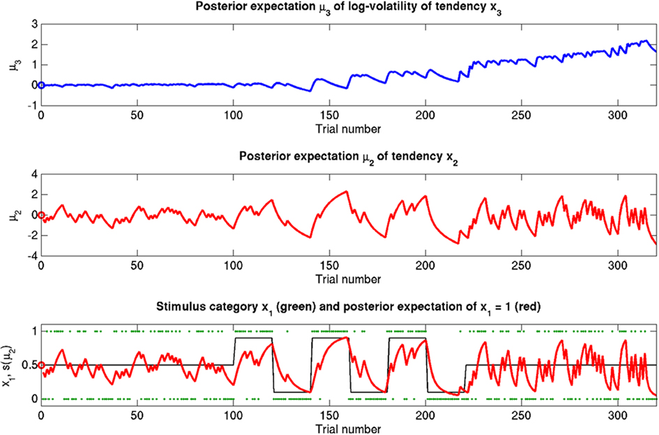
Figure 5. Reference scenario: ϑ = 0.5, ω = −2.2, κ = 1.4. A simulation of 320 trials. Bottom: the first level. Input u is represented by green dots. In the absence of perceptual uncertainty, this corresponds to x1. The fine black line is the true probability (unknown to the agent) that x1 = 1. The red line shows s(μ2); i.e., the agent’s posterior expectation that x1 = 1. Given the input and update rules, the simulation is uniquely determined by the value of the parameters ϑ, ω, and κ. Middle: the second level with the posterior expectation μ2 of x2. Top: the third level with the posterior expectation μ3 of x3. In all three panels, the initial values of the various μ are indicated by circles at trial k = 0.
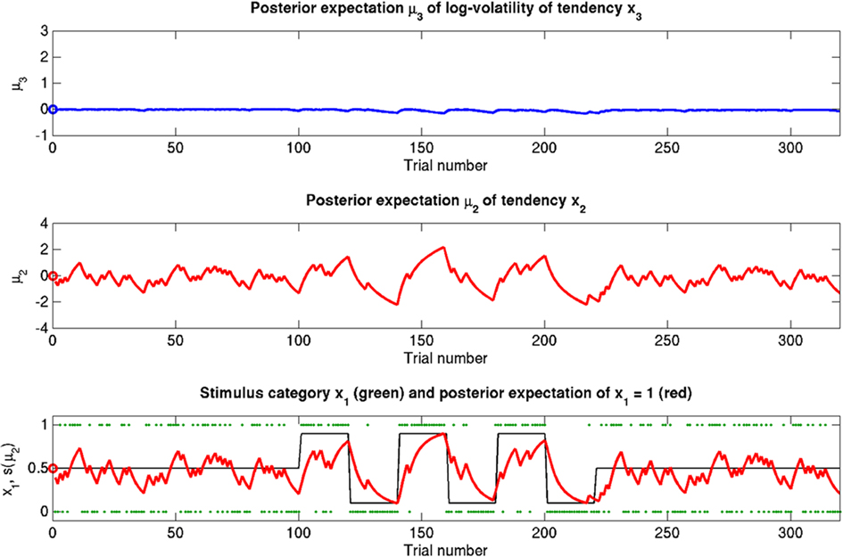
Figure 6. Reduced ϑ = 0.05 (unchanged ω = −2.2, κ = 1.4). Symbols have the same meaning as in Figure 5. Here, the expected x3 is more stable. The learning rate in x2 is initially unaffected but owing to more stable x3 it no longer increases after the period of increased volatility.
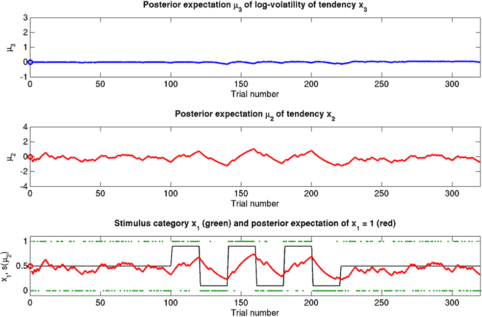
Figure 7. Reduced ω = −4 (unchanged ϑ = 0.5, κ = 1.4). Symbols have the same meaning as in Figure 5. The small learning rate in x2 leads to an extremely stable expected x3. Despite prediction errors, the agent makes only small updates to its beliefs about its environment.
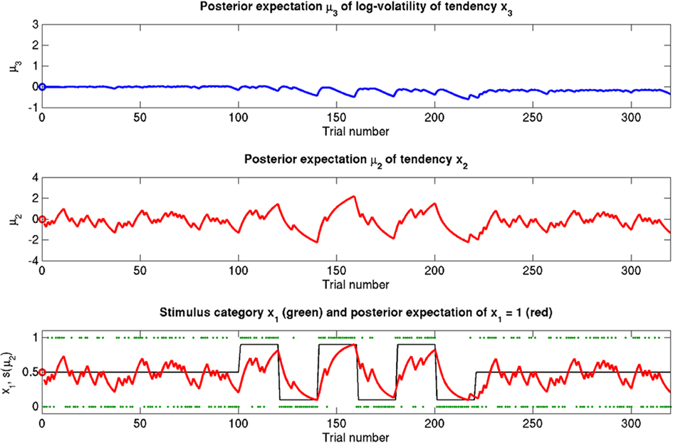
Figure 8. Reduced κ = 0.2 (unchanged ϑ = 0.5, ω = −2.2). Symbols have the same meaning as in Figure 5. x2 and x3 are only weakly coupled. Despite uncertainty about x3, only small updates to μ3 take place. Sensitivity to changes in volatility is reduced. x2 is not affected directly, but its learning rate does not increase with volatility.
The reference scenario in Figure 5 (and Figure 9, top row) illustrates some basic features of the model and its update rules. For this reference, we chose the following parameter values: ϑ = 0.5, ω = −2.2, and κ = 1.4. Overall, the agent is exposed to 320 sensory outcomes (stimuli) that are administered in three stages. In a first stage, it is exposed to 100 trials where the probability that x1 = 1 is 0.5. The posterior expectation of x1 accordingly fluctuates around 0.5 and that of x2 around 0; the expected volatility remains relatively stable. There then follows a second period of 120 trials with higher volatility, where the probability that x1 = 1 alternates between 0.9 and 0.1 every 20 trials. After each change, the estimate of x1 reliably approaches the true value within about 20 trials. In accordance with the changes in probability, the expected outcome tendency x2 now fluctuates more widely around zero. At the third level, the expected log-volatility x3 shows a tendency to rise throughout this period, displaying upward jumps whenever the probability of an outcome changes (and thus x2 experiences sudden updates). As would be anticipated, the expected log-volatility declines during periods of stable outcome probability. In a third and final period, the first 100 trials are repeated in exactly the same order. Note how owing to the higher estimate of volatility (i.e., greater  ), the learning rate has increased, now causing the same sequence of inputs to have a greater effect on μ2 than during the first stage of the simulation. As expected, a more volatile environment leads to a higher learning rate.
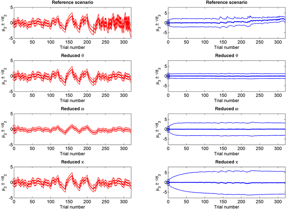
Figure 9. Simulations including standard deviations of posterior distributions. Top to bottom: the four scenarios from Figure 5–8. Left: μ2 (bold red line); fine red lines indicate the range of  around μ2. Right: μ3 (bold blue line); fine blue lines indicate the range
  of around μ3. Circles indicate initial values.
One may wonder why, in the third stage of the simulation, the expected log-volatility μ3 continues to rise even after the true x2 has returned to a stable value of 0 (corresponding to p(x1 = 1) = 0.5; see the fine black line in Figure 5). This is because a series of three x1 = 1 outcomes, followed by three x1 = 0 could just as well reflect a stable p(x1 = 1) = 0.5 or a jump from p(x1 = 1) = 1 to p(x1 = 1) = 0 after the first three trials. Depending on the particular choice of parameters ϑ, ω, and κ, the agent shows qualitatively different updating behavior: Under the parameters in the reference scenario, it has a strong tendency to increase its posterior expectation of volatility in response to unexpected stimuli. For other parameterizations (as in the scenarios described below), this is not the case. Importantly, this ambiguity disappears once the model is inverted by fitting it to behavioral data (see Discussion).
The nature of the simulation in Figure 5 is not only determined by the choice of values for the parameters ϑ, ω, and κ, but also by initial values for μ2, σ2, μ3, and σ3 (the initial value of μ1 is s(μ2)). Any change in the initial value  of μ3 can be neutralized by corresponding changes in κ and ω. We may therefore assume
  without loss of generality but remembering that κ and ω are only unique relative to this choice. However, the initial values of μ2, σ2, and σ3 are, in principle, not neutral. They are nevertheless of little consequence in practice since, when chosen reasonably, they let the time series of hidden states x(k) quickly converge to values that do not depend on the choice of initial value to any appreciable extent. In the simulations of Figures 5–8, we used
 and
and 
If we reduce ϑ (the log-volatility of x3) from 0.5 in the reference scenario to 0.05, we find an agent which is overly confident about its prior estimate of environmental volatility and expects to see little change (Figure 6; Figure 9, second row). This leads to a greatly diminished learning rate for x3, while learning in x2 is not directly affected. There is, however, an indirect effect on x2 in that the learning rate at the second level during the third period is no longer noticeably increased by the preceding period of higher volatility. In other words, this agent shows superficial (low-level) adaptability but has higher-level beliefs that remain impervious to new information.
Figure 7 (and Figure 9, third row) illustrate the effect of reducing ω, the absolute (i.e., independent of x3) component of log-volatility, to −4. The multiplicative scaling exp(ω) of volatility is thus reduced to a sixth of that in the reference scenario. This leads to a low learning rate for x2, which in turn leads to little learning in x3, since the agent can only infer changes in x3 from changes in x2 (cf. Eq. 30). This corresponds to an agent who pays little attention to new information, effectively filtering it out at an early stage.
The coupling between x2 and x3 can be diminished by reducing the value of κ, the relative (i.e., x3-dependent) scaling of volatility in x2 (κ = 0.2 in Figure 8; Figure 9, bottom row). This impedes the flow of information up the hierarchy of levels in such a way that the agent’s belief about x3 is effectively insulated from the effects of prediction error in x2 (cf. Eq. 30). This leads to less learning about x3 and to a much larger posterior variance σ3 than in any of the above scenarios (see Figure 9, right panel). As with a reduced ϑ (Figure 6), learning about x2 itself is not directly affected, except that, in the second stage of the simulation, higher volatility remains without effect on the learning rate of x2 in the third stage. This time, however, this effect is not caused by overconfidence about x3 (due to small ϑ) as in the above scenario. Instead, it obtains despite uncertainty about x3 (large σ3), which would normally be expected to lead to greater learning because of the dependency of the learning rate on σ3. This paradoxical effect can be understood by examining Eqs 30 and 29, where smaller κ exerts opposite direct and indirect effects on the learning rate for μ3. Indirectly, the learning rate is increased, in that smaller κ increases σ3. But this is dominated by the dependency of the learning rate on κ, which leads to a decrease in learning for smaller κ. This is quite an important property of the model: it makes it possible to have low learning rates in a highly volatile environment. This scenario describes an agent which is keen to learn but fails because the levels of its model are too weakly coupled for information to be passed efficiently up the hierarchy. In other words, the agent’s low-level adaptability is accompanied by uncertainty about higher-level variables (i.e., volatility), leading to inflexibility. In anthropomorphic terms, one might imagine a person who displays rigid behavior because he/she remains uncertain about how volatile the world is (e.g., in anxiety disorders).
The simulations described above switch between two probability regimes: p(x1 = 1) = 0.5 and p(x1 = 1) = 0.9 or 0.1. The stimulus distributions under these two regimes have different variances (or risk). Figure 10 shows an additional simulation run where risk is constant, i.e., p(x1 = 1) = 0.85 or 0.15, throughout the entire simulation. One recovers the same effects as in the reference scenario. We now consider generalizations of the generative model that relax some of the simplifying assumptions about sensory mappings and outcomes we made during its exposition above.
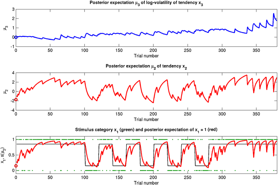
Figure 10. A simulation where risk is constant (ϑ = 0.2, ω = −2.3, κ = 1.6). Symbols have the same meanings as in Figure 5. The same basic phenomena shown in Figure 5 can be observed here.
Perceptual Uncertainty
The model can readily accommodate perceptual uncertainty at the first level. This pertains to the mapping from stimulus category x1 to sensory input u. To allow for perceptual uncertainty, for example when the sensory inputs are ambiguous or affected by noise, we replace the deterministic relation in Eq. 1 by a stochastic one (cf. Daunizeau et al., 2010b):

Here, the input u is no longer binary but a real number whose distribution is a mixture of Gaussians. If x1 = 1, the probability of u is normally distributed with constant variance a around a constant value ηa, corresponding to the most likely sensation if x1 = 1. If, however, x1 = 0, the most likely sensation is ηb with the probability of u normally distributed with the same variance α. The greater a (relative to the squared distance (ηa − ηb)2), the greater the perceptual uncertainty. The main point here is that with this modification, the model can account for situations where x1 can no longer be inferred with certainty from u. The variational energy of the first level now is
With Eq. 15, we find the update rule for μ1:
If u(k) ≈ ηa, one sees that  regardless of
  Likewise,
  if u(k) ≈ ηb. This means that if the sensory input is sufficiently discriminable, x2 has no influence on the agent’s belief about x1. If, however, the sensory input is ambiguous in that u(k) is far from both ηa and ηb (rendering all exponential terms similarly small) we have
  i.e., the agent has to rely on its belief about x2 to predict stimulus category. Importantly, the update equations for the higher levels of the model are not affected by this introduction of perceptual uncertainty at the first level.
Inference on Continuous-Valued States
A generative model that comprises a hierarchy of Gaussian random walks can be applied to many problems of learning and inference. Here, we provide a final example, where the bottom-level state being inferred is not binary but continuous (i.e., a real number). Our example concerns the exchange rate between the U.S. Dollar (USD) and the Swiss Franc (CHF) during the first 180 trading days of the year 2010 (source: http://www.oanda.com). In this example, the agent represented by our model can be seen as an individual market observer (e.g., a currency trader), with the model describing how he “perceives” the relative value (and volatility) of USD. To maintain notational continuity with the preceding sections, we call this value x2 even though it occupies the lowest level of the hierarchy. In other words, the input u is generated directly from x2 (without passing through a binary state x1). The data u are taken to be the closing USD–CHF exchange rates of each trading day with a likelihood model

where a is the constant variance with which the input u is normally distributed around the true value x2. This can be regarded as a measure of uncertainty (i.e., how uncertain the trader is about his “perception” of USD value relative to CHF). On top of this input level, we can now add as many coupled random walks as we please. For our example, we can describe the hidden states in higher levels with Eqs 4 and 5. By the method introduced above, we obtain
For α = 0 (no perceptual uncertainty), the last two equations reduce, as they should, to 
 Note also that since I(x2) is already quadratic here, no further approximation to the mean-field approximation is needed, and μ2 and σ2 are the exact moments of the posterior under the mean-field approximation. Because the higher levels remain the same, the update equations for μ3 and σ3 are as given in Eqs 29 and 30.
Scenarios with different parameter values for the USD–CHF example are presented in Figures 11–14. These scenarios can be thought of as corresponding to different individual traders who receive the same market data but process them differently. The reference scenario (Figure 11) is based on the parameter values κ = 1, ω = −12, ϑ = 0.3, and α = 2·10−5. This parameterization conveys a small amount of perceptual uncertainty that leads to minor but visible deviations of μ2 from u. The updates to μ2 are conservative in the sense that they consider prior information along with new input. Note also that μ3 rises whenever the prediction error about x2 is large, that is when the green dots denoting u are outside the range  indicated by the red lines. Conversely, μ3 falls when predictions of x2 are more accurate. In the next scenario (Figure 12), the value of α is further reduced to 10−6. This scenario thus shows an agent who is effectively without perceptual uncertainty. As prescribed by the update equations above, μ2 now follows u with great accuracy and μ3 tracks the amount of change in x2. In Figure 13, perceptual uncertainty is increased by two orders of magnitude (α = 10−4). Here, the agent adapts more slowly to changes in the exchange rate since it cannot be sure whether prediction error is due to a change in the true value of x2 or to misperception. The final scenario in Figure 14 shows an agent with the same perceptual uncertainty as in the reference scenario but a prior belief that the environment is not very volatile, i.e., ϑ is reduced from 0.3 to 0.01. Smaller values of ϑ smooth the trajectory of μ3 in a similar way that perceptual uncertainty smoothes the trajectory of μ2.
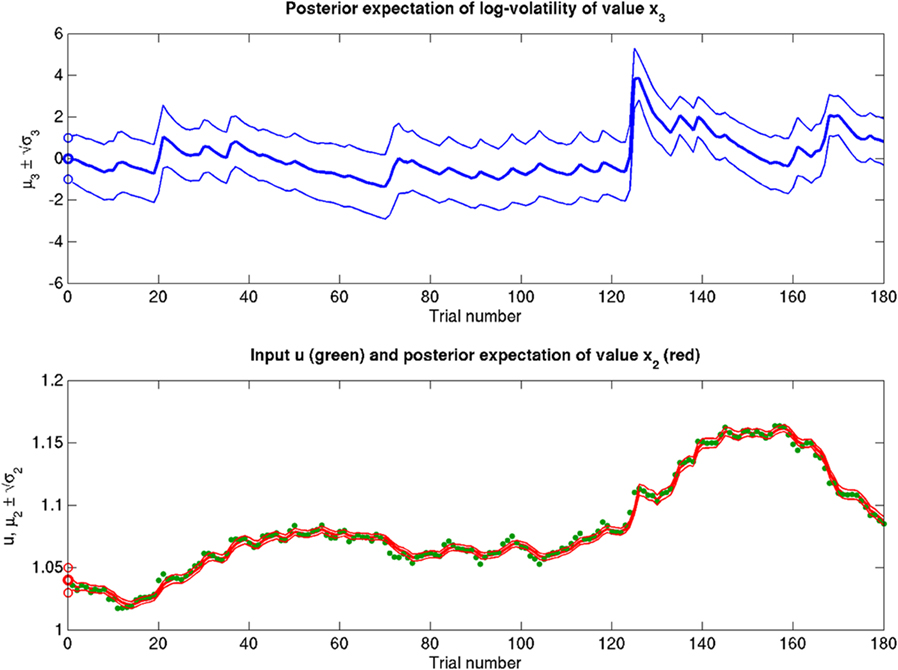
Figure 11. Inference on a continuous-valued state (ϑ = 0.3, ω = −12, κ = 1, α = 2·10−5). Reference scenario for the model of hierarchical Gaussian random walks applied to a continuous-valued state at the bottom level. The state is the value x2 of the U.S. Dollar against the Swiss Franc during the first 180 trading days of the year 2010. Bottom panel: input u representing closing exchange rates (green dots). The bold red line surrounded by two fine red lines indicates the range  . Top panel: The range
  of the log-volatility x3 of x2.
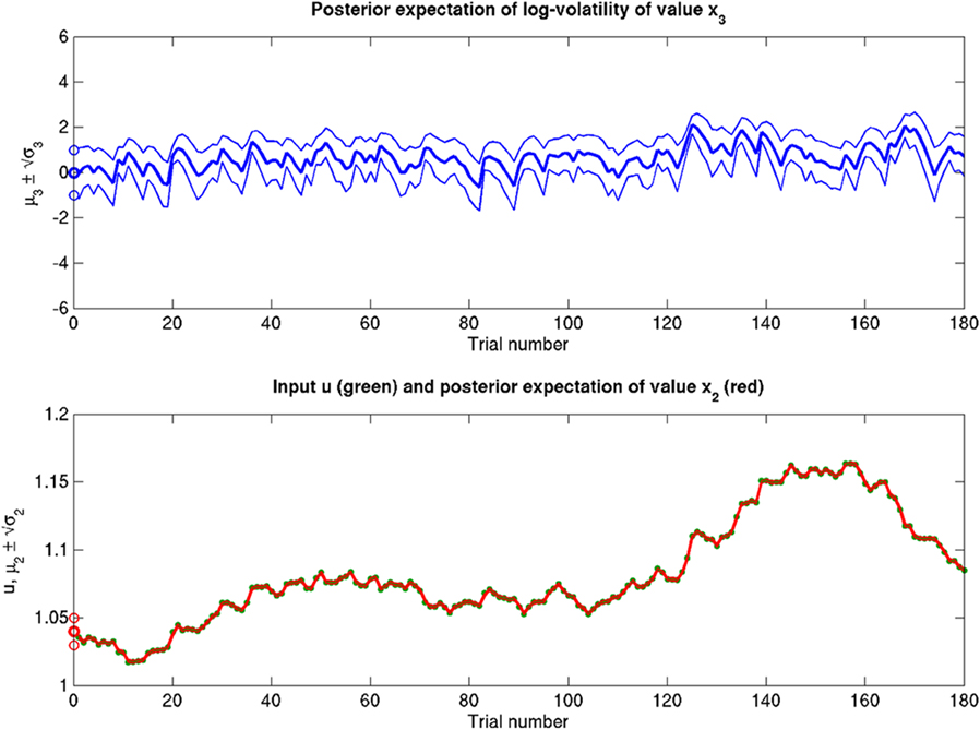
Figure 12. Reduced α = 10−6 (ϑ = 0.3, ω = −12, κ = 1). Reduced perceptual uncertainty α with respect to the reference scenario of Figure 11.
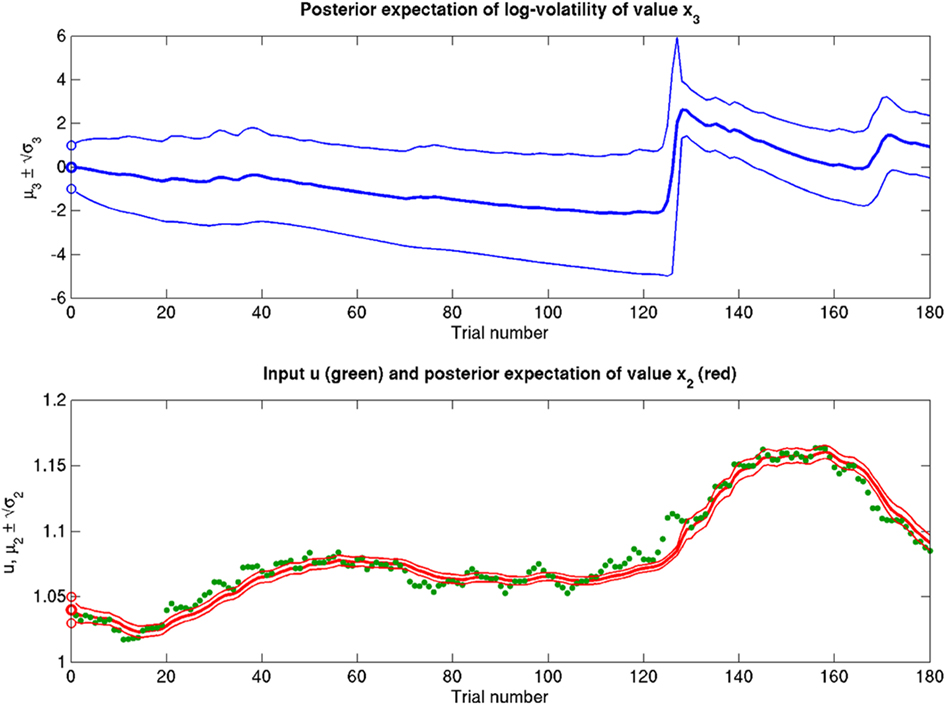
Figure 13. Increased α = 10−4 (ϑ = 0.3, ω = −12, κ = 1). Increased perceptual uncertainty a with respect to the reference scenario of Figure 11.
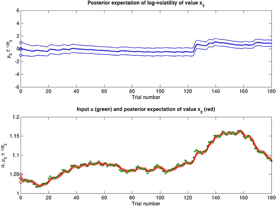
Figure 14. Reduced ϑ = 0.01 (ω = −12, κ = 1, α = 2·10−5). Reduced ϑ with respect to the reference scenario of Figure 11.
This example again emphasizes the fact that Bayes-optimal behavior can manifest in many diverse forms. The different behaviors emitted by the agents above are all optimal under their implicit prior beliefs encoded by the parameters that control the evolution of high-level hidden states. Clearly, it would be possible to optimize these parameters using the same variational techniques we have considered for the hidden states. This would involve optimizing the free energy bound on the evidence for each agent’s model (prior beliefs) integrated over time (i.e., learning). Alternatively, one could optimize performance by selecting those agents with prior beliefs (about the parameters) that had the best free energy (made the most accurate inferences over time). Colloquially, this would be the difference between training an expert to predict financial markets and simply hiring experts whose priors were the closest to the true values. We will deal with these issues of model inversion and selection in forthcoming work (Mathys et al., in preparation). We close this article with a discussion of the neurobiology behind variations in priors and the neurochemical basis of differences in the underlying parameters of the generative model.
Discussion
In this article, we have introduced a generic hierarchical Bayesian framework that describes inference under uncertainty; for example, due to environmental volatility or perceptual uncertainty. The model assumes that the states evolve as Gaussian random walks at all but the first level, where their volatility (i.e., conditional variance of the state given the previous state) is determined by the next highest level. This coupling across levels is controlled by parameters, whose values may differ across subjects. In contrast to “ideal” Bayesian learning models, which prescribe a fixed process for any agent, this allows for the representation of inter-individual differences in behavior and how it is influenced by uncertainty. This variation is cast in terms of prior beliefs about the parameters coupling hierarchical levels in the generative model.
A major goal of our work was to eschew the complicated integrals in exact Bayesian inference and instead derive analytical update equations with algorithmic efficiency and biological plausibility. For this purpose, we used an approximate (variational) Bayesian approach, under a mean-field assumption and a novel approximation to the posterior energy function. The resulting single-step, trial-by-trial update equations have several important properties:
(i) They have an analytical form and are extremely efficient, allowing for real-time inference.
(ii) They are biologically plausible in that the mathematical operations required for calculating the updates are fairly basic and could be performed by single neurons (London and Hausser, 2005; Herz et al., 2006).
(iii) Their structure is remarkably similar to update equations from standard RL models; this enables an interpretation that places RL heuristics, such as learning rate or prediction error, in a principled (Bayesian) framework.
(iv) The model parameters determine processes, such as precision-weighting of prediction errors, which play a key role in current theories of normal and pathological learning and may relate to specific neuromodulatory mechanisms in the brain (see below).
(v) They can accommodate states of either discrete or continuous nature and can deal with deterministic and probabilistic mappings between environmental causes and perceptual consequences (i.e., situations with and without perceptual uncertainty).
Crucially, the closed-form update equations do not depend on the details of the model but only on its hierarchical structure and the assumptions on which the mean-field and quadratic approximation to the posteriors rest. Our method of deriving the update equations may thus be adopted for the inversion of a large class of models. Above, we demonstrated this anecdotally by providing update equations for two extensions of the original model, which accounted for sensory states of a continuous (rather than discrete) nature and perceptual uncertainty, respectively.
As alternatives to our variational scheme, one could deal with the complicated integrals of Bayesian inference by sampling methods or avoid them altogether and use simpler RL schemes. We did not pursue these options because we wanted to take a principled approach to individual learning under uncertainty; i.e., one that rests on the inversion of a full Bayesian generative model. Furthermore, we wanted to avoid sampling approximations because of the computational burden they impose. Although it is conceivable that neuronal populations could implement sampling methods, it is not clear how exactly they would do that and at what temporal and energetic cost (Yang and Shadlen, 2007; Beck et al., 2008; Deneve, 2008).
We would like to emphasize that the examples of update equations derived here can serve as the building blocks for those of more complicated models. For example, if we have more than two categories at the first level, this can be accommodated by additional random walks at the second and subsequent levels; at those levels, Eqs 38 and 40 have a straightforward interpretation in n dimensions. Inference using our update scheme is thus possible on n-categorical discrete states, n-dimensional unbounded continuous states, and (by logarithmic or logistic transformation of variables) n-dimensional bounded continuous states.
One specific problem that has been addressed with Bayesian methods in the recent past concerns online inference of “changepoints,” i.e., sudden changes in the statistical structure of the environment (Corrado et al., 2005; Fearnhead and Liu, 2007; Krugel et al., 2009; Nassar et al., 2010; Wilson et al., 2010). Our generative model based on hierarchically coupled random walks describes belief updating without representing such discrete changepoints explicitly. As illustrated by the simulations in Figures 5–8, this does not diminish its ability to deal with volatile environments. See also previous studies where similar models were applied to data generated by changepoint models (Behrens et al., 2007, 2008) or where RL-type update models were equipped with an adjustable learning rate in order to deal with sudden changes in the environment (Krugel et al., 2009; Nassar et al., 2010). One such sudden change in the environment that is nicely picked up in the application of our model to the empirical exchange rate data is the outbreak of the Greek financial crisis in spring 2010. The sudden realization of the financial markets that Greece was insolvent led to a flight into the USD which is reflected by a sharply increasing value of the Dollar against the Swiss Franc visible in the lower panel of Figure 11. Because this sudden rise of the Dollar is unexpected, it immediately leads to a jump in the agent’s belief about the volatility of its environment, as is clearly visible in the upper panel of Figures 11 or 13. In this manner, a sudden event akin to a changepoint is detected without representations of changepoints being an explicit component of the model.
Clearly, our approach is not the first that has tried to derive tractable update equations from the full Bayesian formulation of learning. Although not described in this way in the original work, even the famous Kalman filter can be interpreted as a Bayesian scheme with RL-like update properties but is restricted to relatively simple (non-hierarchical) learning processes in stable environments (Kalman, 1960). Notably, none of the previous Bayesian learning models we know leads to analytical one-step update equations without resorting to additional assumptions that are specifically tailored for the update equations (Nassar et al., 2010) or the learning rate (Krugel et al., 2009). In contrast, in our scheme, the update equations and their critical components, such as learning rate or prediction error, emerge naturally by inverting a full Bayesian generative model of arbitrary hierarchical depth under a generic mean-field reduction. That is, once we have specified the nature of our approximate inversion, the update equations are fully defined and do not require any further assumptions. This distinguishes our framework conceptually and mathematically from any previously suggested approach to Bayesian learning we are aware of.
Our update scheme also has its limitations. The most important of these is that it depends on the variational energies being approximately quadratic. If they are not, the approximate posterior implied by our update equations might bear little resemblance (e.g., in terms of Kullback–Leibler divergence) to the true posterior. Specifically, the update fails if the curvature of the variational energy at the expansion point is negative (which implies that the conditional variance is negative; see Eq. 38). According to the update Eq. 22, σ2 can never become negative; σ3 = 1/π3 however could become negative according to Eq. 29. However, the simulations and application to empirical (exchange rate) data in this paper suggest that this is not a problem in practice. We are currently investigating the properties of our scheme more systematically in a series of theoretical and empirical analyses that will be published in future work. In particular, we will compare our variational inversion scheme against other methods such as numerical integration and sampling-based methods.
In addition to the derivation of these update equations, we have provided simulations that demonstrate model behavior under different parameterizations (priors). These simulations confirmed the computational efficiency of our approach: the simulations in Figures 5–8 (with 320 trials) each take about 5 ms on a standard laptop computer. Furthermore, they demonstrate that changes in any of the parameters lead to plausible changes in the evolution of the states (i.e., as predicted from the structure of the model) and that each parameter produces distinctly different behavior.
Maladaptive behavior, owing to inappropriate learning and decision-making, is at the heart of most psychiatric diseases, and our framework may be particularly useful for modeling the underlying mechanisms. There are two complementary approaches one might consider: phenomenological and neurophysiological. To illustrate a phenomenological approach, we will consider extreme settings of the parameters in terms of psychopathology. In the example of Figures 5–8, variations in the parameters can explain a spectrum of different types of inference, some of which may be interpreted as aberrant or even pathological. Given the scenario in Figure 8, we could adopt an anthropomorphic interpretation of the agent and interpret underconfidence about estimates of environmental volatility (i.e., high σ3) as a possible cause of anxiety. In other words, knowing that the world is changing quickly is frightening enough, but being uncertain about the extent of this change may be even more upsetting. Anxiety of this sort is often observed prior to (or in the early phase of) psychotic episodes (Häfner et al., 1998). One way to reduce anxiety (that is, to reduce the effects of high s3 due to abnormally low κ), would be to reduce ϑ, leading to a scenario akin to that in Figure 6. This, however, would induce a rigid high-level belief that is impervious to prediction error from the lower level. Rigid high-level priors of this sort that provide inappropriate predictions for lower levels may provide a metaphor for delusions and hallucinations that constitute the positive symptoms of schizophrenia. In contrast, negative symptoms could be related to the scenario in Figure 7: here, a reduction in ω renders the agent completely passive, such that new information is barely taken in and only weakly processed. Notably, in these simple and anecdotal simulations, we chose some parameter settings that lead to superficially similar behavior (e.g., Figures 6 and 8). While this indicates some degree of interdependence among the parameters, this does not mean that the parameters are non-identifiable. Informally, one can intuit this by noting the obvious differences expressed in the evolution of higher-level states of the model; these will be expressed in different behavioral predictions, given a suitably chosen sequence of stimuli. When fitting the model to empirical data, once can test for parameter identifiability more formally using a sensitivity analysis or, equivalently but more conveniently, their posterior covariance. The identifiability of our model parameters will be examined systematically in forthcoming work (Mathys et al., in preparation).
From a neurophysiological perspective, it has been proposed that dopamine might not encode the prediction error on value (Schultz et al., 1997) but instead the value of prediction error, i.e., the precision-weighting of prediction errors (Friston, 2009). In our model, this process is represented, at the second level, by the parameters k and v. It is apparent from the definition Eq. 27 and the update Eq. 22 that these parameters influence the precision of the prediction on the next trial, the precision of the posterior belief, and the learning rate. If dopaminergic midbrain activity encodes the conditional (posterior) precision of beliefs, this dopaminergic activity should be reflected by estimates of κ and ω, obtained from behavioral, fMRI, or electrophysiological data. This hypothesis can be tested using neuropharmacological experiments. In short, by harvesting subject-specific parameter estimates for group analyses of physiological measurements, hierarchical generative models (of the sort considered in this work) could be used to test hypotheses about the relations between computational and physiological processes. We are currently pursuing this approach in ongoing research. Alternatively, one can also use our model for analyses at the subject level: the sequence of inferred hidden states, as represented by their sufficient statistics μ and σ, can be used as predictor variables in analyses of fMRI, EEG, or behavioral data to shed light on the neurophysiological correlates of inference and learning (cf. den Ouden et al., 2010).
The distinction between hidden states, which vary in time and are the dynamic components of the agent’s model of the world, and parameters, which are time-invariant and encode stable subject-specific learning styles, is a key component of our model. One might compare this to classical RL models where value estimates (states) are updated dynamically while the learning rate is an invariant parameter. In our case, however, the (implicit) learning rate is dynamic and results from an interaction between states and parameters: the latter determine how higher-level states influence lower-level ones. This effect of the static parameters on dynamic cross-level coupling can be seen directly from the update equations above (e.g., Eqs 23 and 27) and is illustrated in Figures 5 and 10 where the learning rate visibly changes while the parameters are fixed. In other words, subject-specific learning mechanisms, represented by cross-level coupling in our model, have both dynamic (higher-level states) and static (parameters) components in our model.
One could, of course, consider alternative formulations of our model in which individual learning mechanisms, determined by the coupling across levels, are encoded entirely by states. There is a simple reason why we did not pursue this alternative. Clearly, modeling dynamic aspects of learning, such as rapid updating of learning rates, does require a representation involving states (see above). On the other hand, within an individual agent’s brain, the physiological mechanism underlying this coupling must obey some general principles that have been shaped both by (life-long) experience and genetic background (cf. RL depends on individual genotype (Frank et al., 2007, 2009; Krugel et al., 2009)). Such stable subject-specific learning mechanisms could be represented in two ways. One could choose a relatively deep hierarchical model with high-level states that change very slowly. Alternatively, these mechanisms could be represented by time-invariant parameters. We chose the latter option simply because it provides a more concise and interpretable summary of subject-specific learning mechanisms. For example, when quantifying individual differences in computational learning mechanisms as a function of individual differences in physiology (e.g., pharmacological treatment) or genetics, it is not only statistically easier to deal with time-invariant parameters (i.e., a single number per subject) rather than temporal trajectories of states, but the results are also more readily interpretable.
It should be emphasized that the idea of fitting learning models to subject-specific data and using the ensuing individual parameter estimates for assessing inter-individual variability is not new and has been pursued by many previous studies (e.g., Steyvers and Brown, 2006; Frank et al., 2007, 2009; Krugel et al., 2009). This, however, is less straightforward with those “ideal” Bayesian models that have no free parameters; in this case, parameters can only be taken from adjunct models in which ideal Bayesian models are often embedded (e.g., observation or decision models; cf. Brodersen et al., 2008). The novelty of our approach is that we transform, by variational approximation, an ideal Bayesian learner into a near-optimal scheme in which parameters represent individual learning traits as an integral part of Bayesian learning. These parameters shape the ensuing update equations which are analytical and have an RL-like structure. By combining the principled nature of Bayesian approaches and the practical ease of RL models, we hope that our approach will facilitate future empirical investigations of individual variability.
The main goal of this paper was to introduce the mathematical basis of our approach and illustrate its functionality. Clearly, the simulations shown in this paper are anecdotal and cannot fully demonstrate or establish the practical utility of our approach. In particular, we have not yet demonstrated how our model can be inverted (fitted), given empirical measurements. This requires extending the present approach with a response model that connects states from the Bayesian learning model to measurable responses of a neurophysiological or behavioral sort (cf. Daunizeau et al., 2010a,b). We will present this extension in future work and demonstrate its use for the analysis of behavioral and neuroimaging data.
In summary, we have introduced a novel and generic framework for approximate Bayesian inference with computationally efficient and interpretable closed-form update equations. Simulations show that our approach is applicable to a range of situations beyond classical RL, including inductive inference on discrete and continuous states and situations with perceptual ambiguity. Crucially, our approach accommodates inter-individual differences, in terms of prior beliefs about key model parameters, and quantifies their computational effects: Some of these parameters may map to neurophysiological (neuromodulatory) mechanisms that have been implicated in the neurobiology of learning and psychopathology. As such, it may be a useful framework for modeling individual differences in behavior and to formally characterize behavioral stereotypes and pathophysiologically distinct subgroups in psychiatric spectrum diseases (Stephan et al., 2009).
Conflict of Interest Statement
The authors declare that the research was conducted in the absence of any commercial or financial relationships that could be construed as a potential conflict of interest.
Acknowledgments
This work was supported by the NCCR “Neural Plasticity and Repair” (CM, KES), the University Research Priority Program “Foundations of Human Social Behavior” at the University of Zurich (KES), the Neurochoice project of the Swiss Systems Biology initiative SystemsX.ch (JD, KES), and the Wellcome Trust (KJF).
References
Beal, M. J. (2003). Variational Algorithms for Approximate Bayesian Inference. Ph.D. thesis, University College London. Available at: http://www.cse.buffalo.edu/faculty/mbeal/papers/beal03.pdf
Beck, J., Ma, W., Kiani, R., Hanks, T., Churchland, A., Roitman, J., Shadlen, M., Latham, P. E., and Pouget, A. (2008). Probabilistic population codes for Bayesian decision making. Neuron 60, 1142–1152.
Behrens, T. E. J., Hunt, L. T., Woolrich, M. W., and Rushworth, M. F. S. (2008). Associative learning of social value. Nature 456, 245–249.
Behrens, T. E. J., Woolrich, M. W., Walton, M. E., and Rushworth, M. F. S. (2007). Learning the value of information in an uncertain world. Nat. Neurosci. 10, 1214–1221.
Bresciani, J., Dammeier, F., and Ernst, M. O. (2006). Vision and touch are automatically integrated for the perception of sequences of events. J. Vis. 6, 554–564.
Brodersen, K. H., Penny, W. D., Harrison, L. M., Daunizeau, J., Ruff, C. C., Duzel, E., Friston, K. J., and Stephan, K. E. (2008). Integrated Bayesian models of learning and decision making for saccadic eye movements. Neural Netw. 21, 1247–1260.
Corrado, G. S., Sugrue, L. P., Sebastian Seung, H., and Newsome, W. T. (2005). Linear-nonlinear-poisson models of primate choice dynamics. J. Exp. Anal. Behav. 84, 581–617.
Daunizeau, J., den Ouden, H. E. M., Pessiglione, M., Kiebel, S. J., Stephan, K. E., and Friston, K. J. (2010a). Observing the observer (I): meta-Bayesian models of learning and decision-making. PLoS ONE 5, e15554. doi: 10.1371/journal.pone.0015555
Daunizeau, J., den Ouden, H. E. M., Pessiglione, M., Kiebel, S. J., Friston, K. J., and Stephan, K. E. (2010b). Observing the observer (II): deciding when to decide. PLoS ONE 5, e15555. doi: 10.1371/journal.pone.0015555
Daw, N. D., O’Doherty, J. P., Dayan, P., Seymour, B., and Dolan, R. J. (2006). Cortical substrates for exploratory decisions in humans. Nature 441, 876–879.
Dayan, P., and Niv, Y. (2008). Reinforcement learning: the good, the bad and the ugly. Curr. Opin. Neurobiol. 18, 185–196.
den Ouden, H. E. M., Daunizeau, J., Roiser, J., Friston, K. J., and Stephan, K. E. (2010). Striatal prediction error modulates cortical coupling. J. Neurosci. 30, 3210–3219.
Fearnhead, P., and Liu, Z. (2007). On-line inference for multiple changepoint problems. J. R. Stat. Soc. Series B Stat. Methodol. 69, 589–605.
Frank, M. J. (2008). Schizophrenia: a computational reinforcement learning perspective. Schizophr. Bull. 34, 1008–1011.
Frank, M. J., Doll, B. B., Oas-Terpstra, J., and Moreno, F. (2009). Prefrontal and striatal dopaminergic genes predict individual differences in exploration and exploitation. Nat. Neurosci. 12, 1062–1068.
Frank, M. J., Moustafa, A. A., Haughey, H. M., Curran, T., and Hutchison, K. E. (2007). Genetic triple dissociation reveals multiple roles for dopamine in reinforcement learning. Proc. Natl. Acad. Sci. U.S.A. 104, 16311–16316.
Friston, K. (2008). Hierarchical models in the brain. PLoS Comput. Biol. 4, e1000211. doi: 10.1371/journal.pcbi.1000211
Friston, K. (2009). The free-energy principle: a rough guide to the brain? Trends Cogn. Sci. (Regul. Ed.) 13, 293–301.
Friston, K., Mattout, J., Trujillo-Barreto, N., Ashburner, J., and Penny, W. (2007). Variational free energy and the Laplace approximation. Neuroimage 34, 220–234.
Geisler, W. S., and Diehl, R. L. (2002). Bayesian natural selection and the evolution of perceptual systems. Philos. Trans. R. Soc. B Biol. Sci. 357, 419–448.
Gershman, S. J., and Niv, Y. (2010). Learning latent structure: carving nature at its joints. Curr. Opin. Neurobiol. 20, 251–256.
Gluck, M. A., Shohamy, D., and Myers, C. (2002). How do people solve the weather prediction task? individual variability in strategies for probabilistic category learning. Learn. Mem. 9, 408–418.
Gu, Q. (2002). Neuromodulatory transmitter systems in the cortex and their role in cortical plasticity. Neuroscience 111, 815–835.
Häfner, H., Maurer, K., Löffler, W., an der Heiden, W., Munk-Jørgensen, P., Hambrecht, M., and Riecher-Rössler, A. (1998). The ABC schizophrenia study: a preliminary overview of the results. Soc. Psychiatry Psychiatr. Epidemiol. 33, 380–386.
Herz, A. V. M., Gollisch, T., Machens, C. K., and Jaeger, D. (2006). Modeling single-neuron dynamics and computations: a balance of detail and abstraction. Science 314, 80–85.
Jaynes, E. T. (2003). Probability Theory: The Logic of Science. Cambridge, UK: Cambridge University Press.
Kalman, R.E. (1960). A new approach to linear filtering and prediction problems. J.Basic Eng. 82, 35–45.
Kording, K. P., and Wolpert, D. M. (2004). Bayesian integration in sensorimotor learning. Nature 427, 244–247.
Krugel, L. K., Biele, G., Mohr, P. N. C., Li, S., and Heekeren, H. R. (2009). Genetic variation in dopaminergic neuromodulation influences the ability to rapidly and flexibly adapt decisions. Proc. Natl. Acad. Sci. U.S.A. 106, 17951–17956.
Laplace, P. (1774). Mémoire sur la probabilité des causes par les évènemens. Mém. Acad. Roy. Sci. 6, 621–656.
Montague, P. R., Hyman, S. E., and Cohen, J. D. (2004). Computational roles for dopamine in behavioural control. Nature 431, 760–767.
Murray, G. K., Corlett, P. R., Clark, L., Pessiglione, M., Blackwell, A. D., Honey, G., Jones, P. B., Bullmore, E. T., Robbins, T. W., and Fletcher, P. C. (2007). Substantia nigra/ventral tegmental reward prediction error disruption in psychosis. Mol. Psychiatry 13, 267–276.
Nassar, M. R., Wilson, R. C., Heasly, B., and Gold, J. I. (2010). An approximately Bayesian delta-rule model explains the dynamics of belief updating in a changing environment. J. Neurosci. 30, 12366–12378.
O’Doherty, J., Dayan, P., Schultz, J., Deichmann, R., Friston, K., and Dolan, R. J. (2004). Dissociable roles of ventral and dorsal striatum in instrumental conditioning. Science 304, 452–454.
Orbán, G., Fiser, J., Aslin, R. N., and Lengyel, M. (2008). Bayesian learning of visual chunks by human observers. Proc. Natl. Acad. Sci. U.S.A. 105, 2745–2750.
Pessiglione, M., Seymour, B., Flandin, G., Dolan, R. J., and Frith, C. D. (2006). Dopamine-dependent prediction errors underpin reward-seeking behavior in humans. Nature 442, 1042–1045.
Preuschoff, K., and Bossaerts, P. (2007). Adding prediction risk to the theory of reward learning. Ann. N. Y. Acad. Sci. 1104, 135–146.
Rescorla, R. A., and Wagner, A. R. (1972). “A theory of Pavlovian conditioning: Variations in the effectiveness of reinforcement,” in Classical Conditioning II: Current Research and Theory, eds A. H. Black and W. F. Prokasy (New York: Appleton-Century-Crofts), 64–99.
Schultz, W., Dayan, P., and Montague, P. R. (1997). A neural substrate of prediction and reward. Science 275, 1593–1599.
Smith, A., Li, M., Becker, S., and Kapur, S. (2006). Dopamine, prediction error and associative learning: a model-based account. Network 17, 61–84.
Stephan, K. E., Friston, K. J., and Frith, C. D. (2009). Dysconnection in schizophrenia: from abnormal synaptic plasticity to failures of self-monitoring. Schizophr. Bull. 35, 509–527.
Steyvers, M., and Brown, S. (2006). Prediction and change detection. Adv. Neural Inf. Process Syst. 18, 1281–1288.
Steyvers, M., Lee, M. D., and Wagenmakers, E. (2009). A Bayesian analysis of human decision-making on bandit problems. J. Math. Psychol. 53, 168–179.
Sutton, R. S., and Barto, A. G. (1998). Reinforcement Learning: An Introduction. Cambridge, MA: MIT Press.
Thiel, C. M., Huston, J. P., and Schwarting, R. K. (1998). Hippocampal acetylcholine and habituation learning. Neuroscience 85, 1253–1262.
Wilson, R. C., Nassar, M. R., and Gold, J. I. (2010). Bayesian online learning of the hazard rate in change-point problems. Neural. Comput. 22, 2452–2476.
Xu, F., and Tenenbaum, J. B. (2007). Sensitivity to sampling in Bayesian word learning. Dev. Sci. 10, 288–297.
Keywords: hierarchical models, variational Bayes, neuromodulation, dopamine, acetylcholine, serotonin, decision-making, volatility
Citation: Mathys C, Daunizeau J, Friston KJ and Stephan KE (2011) A Bayesian foundation for individual learning under uncertainty. Front. Hum. Neurosci. 5:39. doi: 10.3389/fnhum.2011.00039
Received: 01 January 2011;
Accepted: 29 March 2011;
Published online: 02 May 2011.
Edited by:
Sven Bestmann, University College London, UKReviewed by:
Quentin Huys, University College London, UKRobert C. Wilson, Princeton University, USA
Copyright: © 2011 Mathys, Daunizeau, Friston and Stephan. This is an open-access article subject to a non-exclusive license between the authors and Frontiers Media SA, which permits use, distribution and reproduction in other forums, provided the original authors and source are credited and other Frontiers conditions are complied with.
*Correspondence: Christoph Mathys, Laboratory for Social and Neural Systems Research, Department of Economics, University of Zurich, Bluemlisalpstrasse 10, 8006 Zurich, Switzerland. e-mail: chmathys@ethz.ch