Three-dimensional brain reconstruction of in vivo electrode tracks for neuroscience and neural prosthetic applications

Introduction

The neuroscience field has experienced rapid technological advances over the past decade, including the development of multi-site array technologies that can record or stimulate across more than 100 sites (Lehew and Nicolelis, 2008; Falcone and Bhatti, 2011; Stevenson and Kording, 2011), the discovery of optogenetics in which neurons can be genetically altered to become excited or suppressed to different lights (Bamann et al., 2010; Fenno et al., 2011; Miesenbock, 2011), and advances in magnetic resonance imaging (MRI) techniques that have enabled non-invasive functional and anatomical mapping of the brain (Yacoub et al., 2008; Lenglet et al., 2009; Leergaard et al., 2010; Van Essen et al., 2012). These advances have led to more detailed and intricate studies in understanding how individual neurons interact and function as a network, leading to perception and action. In parallel, there have also been significant developments in brain stimulation approaches for treating various sensory, motor, and neurological disorders (Lozano and Hamani, 2004; Zhou and Greenbaum, 2009; Tierney et al., 2011). Two main examples are deep brain stimulation (DBS) for treating neurological disorders [e.g., Parkinson's or Essential Tremor; >75,000 DBS patients worldwide (Zrinzo et al., 2011)] and central auditory prostheses for hearing restoration [within the brainstem or midbrain; >1000 patients worldwide (Lim et al., 2011)]. The increased knowledge gained from basic neuroscience research has provided some insight into the function of neural circuitry relevant for brain stimulation devices. However, one major bottleneck in successful implementation of these different neural prosthetics has been the identification of optimal locations for stimulation to treat the health condition (Johnson et al., 2008; McCreery, 2008; Lim et al., 2009; Hemm and Wardell, 2010).

Neurophysiology experiments can provide spatial mapping of the brain down to a cellular scale. Thus, it would seem that understanding neural function at a sufficient spatial resolution for identifying appropriate brain locations for prosthetic stimulation would not be a major hurdle. However, neurophysiological studies are not typically accompanied by detailed brain reconstructions identifying the actual locations of the recording and/or stimulation sites. For example, there are over a thousand studies related to auditory coding in the inferior colliculus (IC), the main auditory structure of the midbrain (e.g., using key words “IC” and “auditory” in PubMed). In contrast, there are only a handful of IC neurophysiology studies that provide detailed histological reconstruction of their recording or stimulation site locations (e.g., Merzenich and Reid, 1974; Malmierca et al., 2008; Loftus et al., 2010). Histological confirmation of the sites is typically used to indicate general placement within a nucleus rather than to systematically identify coding features across that nucleus. With the recent developments of an IC-based auditory prosthesis (auditory midbrain implant, AMI), it has become increasingly important to identify which regions of the IC are well-suited for electrical stimulation to restore intelligible hearing (Lim et al., 2007, 2009). Detailed neurophysiological mapping studies with sufficient spatial information are necessary to guide future IC stimulation strategies. Unfortunately, there is no consistent histological method used across labs that enables functional and anatomical data to be pooled across studies to lead to a more spatially complete picture of auditory coding in the IC. These limitations are not only observed in auditory research but throughout the neuroscience field.

Three-dimensional brain reconstruction and modeling is not a new concept, yet is one that needs to be revived in neurophysiology labs, especially as brain stimulation approaches become more widely implemented in patients. MRI techniques have provided a successful pathway for fusing anatomical organization with neural function (Yacoub et al., 2008; Lenglet et al., 2012; Van Essen et al., 2012). However, in parallel, neurophysiological mapping studies are still needed to understand the neural coding features at multiple spatial and time scales, rather than focusing solely on the indirect measure of the slow hemodynamic response captured by functional MRI (Sutton et al., 2009; Glover, 2011). The cellular structure and neurochemical function can also be investigated in stained histological slices and correlated with the neurophysiological mapping results (Cant and Benson, 2005; Dauguet et al., 2007; Bohland et al., 2009; Kleinfeld et al., 2011).

As a step toward bridging the gap between cellular function and network coding organization, especially in identifying appropriate locations within specific nuclei for neural prosthetic applications, we developed a simple and relatively inexpensive three-dimensional brain reconstruction method that uses standard histological techniques and equipment commonly available in research labs. The process uses a three-dimensional rendering software (Rhinoceros, Seattle, WA) that is inexpensive (~$200 for a student version). Although preparing the slices and creating the reconstructions requires a significant time commitment, the entire process is easy to learn and we have been able to recruit volunteer students to perform the reconstructions. The students benefit from this arrangement by participating in the neurophysiology experiments and being provided an initial reconstruction project to learn brain anatomy. Thus in an academic setting, it is possible to perform inexpensive, detailed brain reconstructions to supplement neurophysiology data using this approach.

The overall goal of this method is to establish a relatively simple and accessible standard for how different labs perform brain reconstructions that will be available online and enable data to be pooled across studies. Initially, we investigated our approach for reconstructing the IC due to immediate interests in guiding AMI stimulation strategies. In this paper, we will first present the detailed steps involved with the reconstruction approach in the Methods. The error analysis and the ability to consistently reconstruct electrode tracks and sites positioned across the frequency axis of the IC will then be presented in the Results. Finally, potential improvements and new directions for brain reconstructions will be presented in the Discussion.

Methods

We have developed a reconstruction method combining histological brain slices and neurophysiological recordings to identify the tracks and site locations of acutely implanted electrode arrays in the IC. The detailed steps in performing the brain reconstructions are presented below. Additionally, a video simulation of the entire computer reconstruction process using Rhinoceros can be downloaded from soniclab.umn.edu.

Animal Surgery and Electrode Array Placement

Electrophysiological experiments were performed on young Hartley guinea pigs (Elm Hill Breeding Labs, Chelmsford, MA) under ketamine (40 mg/kg) and xylazine (10 mg/kg) anesthesia in accordance with policies of the University of Minnesota Institutional Animal Care and Use Committee. Further details on the anesthesia and surgical approach have been presented previously (Lim and Anderson, 2007b; Neuheiser et al., 2010) and are only briefly described here. All animals had a mass of 330–380 g at the time of experiment. A silicon-substrate, multi-site Michigan electrode array (Figure 1; NeuroNexus Technologies, Ann Arbor, MI) was acutely implanted into the right IC. The probe consists of two shanks separated by 500 μm, with each shank having 16 iridium sites linearly spaced 100 μm apart (center-to-center). Before placement, the shanks were dipped 10 times in a red fluorescent dye [3 mg Di-I (1,1′-dioctadecyl-3,3,3′,3′-tetramethylindocarbocyanine perchlorate) per 100 μL acetone; Sigma-Aldrich, St. Louis, MO], alternating between 10 s in and 10 s out of the dye. The Di-I is visible in brightfield images of brain slices, fluoresces for added visualization, and has been used successfully in previous studies without noticeably altering neural activity (DiCarlo et al., 1996; Jain and Shore, 2006; Lim and Anderson, 2007b). The probe was stereotaxically inserted at a 45° angle off the sagittal plane through the occipital cortex into the IC, with one shank placed approximately rostral to the other. The 45° angle aligns the probe along the tonotopic axis of the IC, while the bi-shank design allows for simultaneous recordings within isofrequency laminae. The fixed-distance bi-shank design is also crucial for identifying the location of individual electrode sites as described later in the Methods. The probe only needed to be stained prior to the first implantation location and the stained track could be visualized across multiple locations (up to 12 placements corresponding to 24 shank tracks) throughout the entire experiment. Each placement lasted approximately one hour for recording acoustic-driven neural activity that was later used for offline characterization of the functional organization.

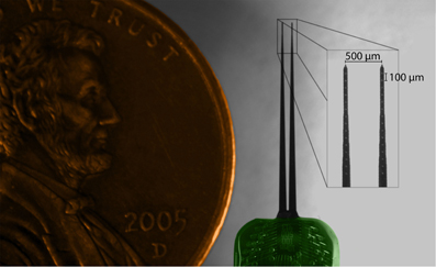
Figure 1. Microscope image of acutely-implanted Michigan electrode array (NeuroNexus Technologies, Ann Arbor, MI) consisting of two shanks (10 mm long) each with 16 contacts (~400 μm² site area) spaced 100 μm apart center-to-center.

Histological Slice Preparation

After our in vivo experiment, the animal was euthanized with an overdose (0.07 mL/mg) of Beuthanasia-D Special (Merck, Summit, NJ) into the heart. The animal was then decapitated and the head was fixed in 3.7% paraformaldehyde and stored in a 4°C refrigerator for 3–6 days, during which time most of the skull overlying the cortex was also removed to increase diffusion of the fixative into the brain. This duration sufficiently fixed the tissue to allow removal of the brain from the skull without damaging its bottom surface, which is used to later align and cut the tissue to extract the midbrain. The brain was immersed in fixative for about three more days after its removal from the skull. Future protocols should include transcardial perfusion to improve fixation of deeper structures, especially when attempting to histologically characterize cellular organization and function. However, based on previous studies (Bledsoe et al., 2003; Lim and Anderson, 2007b; Neuheiser et al., 2010) and as shown later in the Results, this simpler fixation protocol was sufficient to consistently reconstruct our brain tissue and electrode tracks.

To block the midbrain, a custom-made slicing box (specifications found at soniclab.umn.edu) was built to assure straight-edge cuts. Commercial brain blockers have a set mold that the full brain rests in and do not work for slicing partial brain regions, such as the midbrain. The custom slicing box has holes through which the brain can be pinned down and allows the full brain or partial regions to be blocked carefully along appropriate planes. Although this custom-made slicing box was used for the histological preparations in this paper, any preferred apparatus or method can be used to make straight-edge cuts. This slicing box was originally designed and used to increase the consistency in how different midbrains were blocked to improve normalization of data across animals. However, it was frequently observed that anatomical variations between brains could cause them to lie in the box with slightly different orientations, leading to different angled cuts across the edges of the extracted midbrains. Similar cutting issues occur when using commercial brain blockers (e.g., Kopf Instruments, Tujunga, CA). As described in detail in section “Normalizing Across Multiple Midbrains,” a unique solution to this problem has been to identify consistent anatomical landmarks that can be used to align and normalize brains across animals without relying on the sliced edges. The only critical requirement for any slicing apparatus used for blocking the midbrain is that it can create a straight-edge cut along the correct midline of the midbrain important for the normalization procedure.

There are several steps that were used to block the midbrain. Initially, with the brain sitting on its ventral side and pinned down through the frontal lobes and the cerebellum, a coronal cut was made caudal to the cerebellum to remove the back portion of the spinal cord, allowing the brain to sit flat in the box (Figure 2A). Another coronal cut, made through the center of the temporal lobes, removed the rostral half of the brain (Figure 2B), and the cortex was peeled away from the midbrain (Figure 2C). Using a small razor, the cerebellum was then carefully pulled and cut away from the midbrain (Figure 2D). Finally, the left midbrain was pinned down in the box and a sagittal cut was made through the visible midline track to extract the right midbrain (Figure 2E).

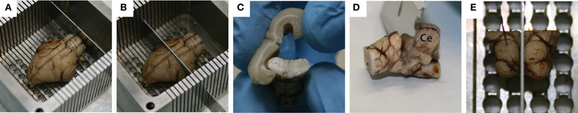
Figure 2. Standard blocking procedure for extracting the midbrain. With the brain pinned to the custom-made slicing box through the frontal lobe and the cerebellum, a coronal slice was made caudal of the cerebellum to remove the spinal cord (A), while a second coronal slice was made through the center of the temporal lobes to remove the rostral half of the brain (B). A frontal view of the cortex being peeled away from the midbrain is shown in (C), followed by removal of the cerebellum (labeled Ce in D) using a small razor. Finally, with the left midbrain pinned down, a mid-sagittal cut was made to extract the right midbrain (E). Red dots on the right inferior colliculus show where the dyed shanks entered through its surface during the in vivo portion of the experiment.

For accurate alignment of the midbrain slices during reconstruction, three reference tracks were created in the lateral-to-medial direction in the right midbrain. With the midbrain resting on its medial edge, a small needle stained with Di-I was stereotaxically inserted perpendicular to the lateral surface and left for 15 min to allow the Di-I to diffuse into the tissue, while dripping a sucrose solution (15 g sucrose per 100 mL of 0.1 M PBS) on the midbrain to keep it moist. The first track was inserted into the intersection point of the superior colliculus (SC), thalamus, and the lateral extension from the IC as shown in Figure 3C (black arrow). This is a consistent anatomical landmark across animals (termed the “consistent reference track”) and is critical for accurate alignment of the slices. As discussed later in the Methods, the lateral edge of this reference track is used to normalize across multiple brains, making its consistent placement vital to the method's success. To avoid misalignments due to slice rotation errors and tearing along the reference track, two additional perpendicular reference tracks were arbitrarily created within the tissue but outside of the IC as to not interfere with the electrode shank placements (gray tracks in Figures 3E and F). It is also possible to create angled reference tracks if angled electrode trajectories are not available to later aid in the alignment process. After creating the three reference tracks, the midbrain was placed into a sucrose solution until the tissue sank (~1 day). The midbrain was then dipped in saline and frozen on its medial edge to –18°C for cryosectioning. Sagittal sections (60 μm thickness) were cut using a sliding microtome (Leica, Buffalo Grove, IL) and placed in wells filled with a phosphate buffer (9:1 di-ionized H₂0 to PBS). The slices were dipped in a sodium acetate buffer and mounted onto slides for imaging. Each slice was labeled with the distance from the lateral edge of the IC and any slice with extreme tearing was discarded. Sagittal sectioning ensured that each slice showed a single point for each electrode track (placed at a 45° angle off the sagittal plane) and reference track (placed at a 90° angle off the sagittal plane).

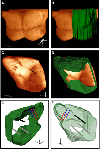
Figure 3. Histological computer reconstruction of the midbrain overlaid on a top view (A,B) and lateral view (C,D) of the fixed midbrain. Images were digitally enhanced to improve visualization of the borders. The reconstructed midbrain was also slanted in A and B to align it with the angled view of the fixed midbrain, which was purposely presented in this way to visualize the lateral side of the right inferior colliculus. The placement of the “consistent reference track,” which is through the intersection of the superior colliculus, thalamus, and lateral extension from the inferior colliculus, is indicated by the black arrow in (C). Computer reconstructions are rotated to view them from the medial (E) and lateral (F) sides. The consistent reference track is shown in black, the two arbitrarily-placed reference points are in gray, and the two bi-shank probe pairs are in red and blue. C, caudal; D, dorsal; L, lateral.

Imaging of Sections

Slice images were taken within a week of sectioning using a Leica MZ FLIII fluorescent stereomicroscope (Leica, Buffalo Grove, IL), Leica DFC420 C peltier cooled CCD camera, and Image-Pro software (MediaCybernetics, Bethesda, MD). At least two fluorescent images using a filter set with a 546/10 nm excitation and 590 nm emission were taken of each slice with varying degrees of exposure (Figure 4). Fluorescent images were taken while varying the exposure time (3–3.5 s) and gain (2.5–4×) to optimize the visualization points (i.e., higher values to see dull points, lower values to remove flare in bright points). A single reflective white light image using a variable intensity fiber optic light source (Fiber-Lite-PL800, Dolan-Jenner Industries, Boxborough, MA) was taken to determine the outline of each slice for tracing. Fluorescence images were later superimposed on the reflective white light images for visualization of the reference and electrode shank points. The images were then saved as .tif files and labeled with their distance from the lateral edge of the IC. All images were taken at the same zoom for consistency, and an additional image of a 1 mm scale ruler was taken to later calibrate the image size in the modeling software.

Figure 4. Fluorescent images of the same 60 μm thick sagittal slice with reflective white light (A) and fluorescence (B) settings. Each slice was outlined in white and three reference points (large white circle) and two pairs of electrodes (small white circles) were identified. IC, inferior colliculus; SC, superior colliculus; C, caudal; D, dorsal.

Tracing Images

The .tif images were imported into Rhinoceros, a three-dimensional modeling tool for designers (Seattle, WA). A detailed view of the Rhinoceros interface is shown in Figure 5. Grid lines were placed (major every 100 μm, minor every 10 μm) and the snap spacing was enabled and set to 1 μm. At this point, distances within the Rhinoceros interface were arbitrary, but once all of the images were placed and traced, the 1 mm ruler image was used to scale all of the tracings to the correct physical size. The first bitmap was placed at the origin and a frame was created around the outline to place subsequent bitmaps (Figures 5A and B). Once the frame was in place, grid line snap was turned off and grayscale was turned off to better visualize the slices. Each slice was traced using the InterpolateCurve command, ignoring tears that extended beyond the obvious border of the slice, and saved as a new layer. Any slice with significant tearing or folding was discarded (typically <5% of total slices). Once a reflective white light image outline was traced, the same slice's fluorescence image was overlaid to identify the reference points and shank placements, which were chosen using the Circle command with 3 μm and 1 μm radii, respectively (white circles in Figure 4). Lastly, each completed tracing was moved to the correct sagittal depth based on its distance from the lateral edge of the IC and spaced 60 μm from the neighboring slices assuming no torn slices were removed (Figure 5C).

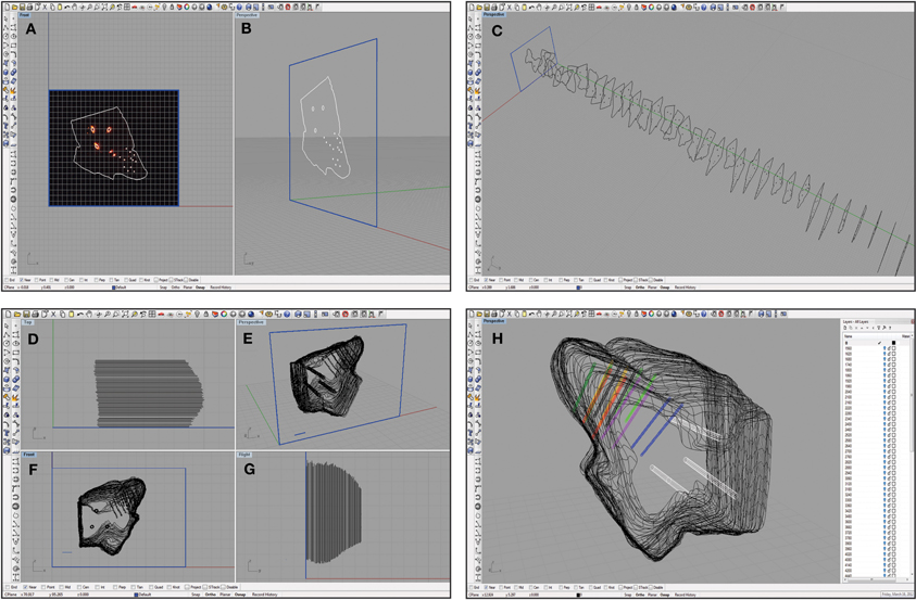
Figure 5. Screen shots of the Rhinoceros software interface at various steps in the reconstruction process. A single slice was placed in a frame of arbitrary size (shown in blue) at the origin and traced as shown from a medial (A) and an oblique (B) view. This process was repeated for each slice that was also placed at the correct location on the medial-to-lateral axis (C). Damaged slices that could not be accurately traced were not included, leaving larger gaps between the surrounding slices. The slices were then aligned using the three reference points as shown from a top view (D), an oblique angle (E), a medial view (F), and from the caudal side (G). Larger spacing in (D) and (G) indicate where torn slices were removed from the reconstruction. These slices were also scaled using a 1 mm ruler (shown in blue; E and F). Finally, the wireframe was meshed using approximately 50 control points around the shell of the midbrain, and the reference points (white) and electrode array tracks (multiple colors; bi-shank probe pairs are color-matched) were meshed to create tube-like trajectories (H). The white menu on the right indicates the number of layers that can be turned on or off to increase visualization of specific features at any given time.

Aligning Slices

With the tracings in the correct position, they needed to be rotated and aligned to each other using the reference tracks and the electrode trajectories. First, the ICs were approximately arranged across slices, and slices that were mounted on the slides backwards were mirrored. The consistent reference track at the intersection of the SC, thalamus, and the lateral extension from the IC was aligned across slices. The tracings were then rotated to align the other two reference tracks through the midbrain and match the straight rostral edge created from the frontal cut during the blocking process (Figures 5D–G). The 45° angled electrode trajectories combined with the three reference tracks provided multiple axes to align all the slices while minimizing shifting of each slice relative to each other. Finally, the image of the 1 mm ruler was imported into Rhinoceros, traced, and used to scale the arbitrary distances within Rhinoceros to the actual physical dimensions of the slices.

Creation of Best Fit Lines for Electrode Tracks

To visualize the complete electrode shank trajectories, we created a best fit line through the electrode shank placements across all the traced slices, examples of which are shown in Figure 5H. To create each best fit line, a new layer in Rhinoceros was created, the center snap feature was turned on, and the points making up a given track were selected across all the slices. Using the LineThroughPt command, a best fit line through all of the points was created and saved as the final trajectory. A similar fitting procedure was also performed for the reference tracks.

Construction of 3D Mesh

With all of the tracings aligned at the correct orientation, they needed to be meshed to create a complete surface. In a new layer, the Loft command in Rhinoceros was used. At least 50 control points were chosen on the outline of the tracings and a mesh was formed around those points. If more control points were selected, the mesh around the tracings became tighter and created a more jagged rendering of the three-dimensional surface. Also, the electrode best fit lines and the reference tracks were meshed for visualization purposes using the Loft command, creating tube-like trajectories (Figure 5H).

Identifying the Location of Electrode Sites

To identify the location of each electrode site along a shank track, a few extra steps and probe requirements were needed. First, during the in vivo portion of the experiment, the electrode array was initially inserted only partially within the IC. Neural activity was recorded on each site in response to 100 trials of 70 dB broadband noise (6 octaves wide centered at 5 kHz). The border of the IC, as shown in Figure 6, was identified as the location halfway between the last site showing a significant response [i.e., >76% correct in a signal detection theory paradigm (Green and Swets, 1966; Lim and Anderson, 2006; Middlebrooks and Snyder, 2007)] and the next superficial site (spaced 100 μm away). The electrode array was then inserted using a hydraulic micro-manipulator into the final location for experimentation, noting the additional distance the array was inserted into the midbrain.

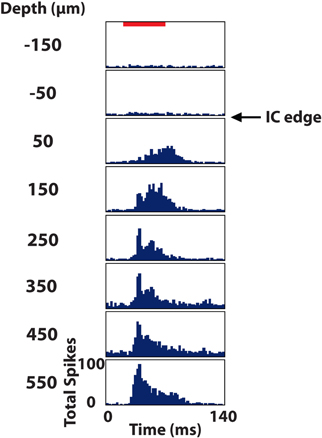
Figure 6. Post stimulus time histograms of eight sites in the inferior colliculus (IC) in response to 100 trials of broadband noise (70 dB SPL, 6 octaves centered at 5 kHz). The red bar corresponds to the acoustic stimulus (60 ms duration) and depths are labeled relative to the superficial edge of the IC, which was approximated as the center point between the last electrode site responding significantly to the stimulus and the next site outside of the IC.

Though the physical distance of each electrode site along a track within the IC was known for the in vivo preparation, the fixation process could cause the midbrain to change in size and modify the track and site locations. To address this issue, an electrode array with two shanks separated by a fixed distance (500 μm apart) was necessary for assessing how much the tissue changed during fixation. Assuming the brain changes size in a homogenous and isotropic manner, it was possible to take the average change in distance between pairs of shanks across all placements throughout the IC for a given animal and use that scaling factor to adjust the distance from the edge of the IC of each site measured in vivo to match the reconstructed IC dimensions. The scale factor across animals showed that the midbrain shrank an average of <4% from its in vivo size. Other studies have observed tissue shrinkage up to 10–15% (Cant and Benson, 2005; Dauguet et al., 2007), which was not observed for the protocol used in this study. The creative use of probes with fixed-shanks can partially correct for morphological changes that occur during the fixation process. Considering recent advances in multi-site array technologies in which three-dimensional configurations with micron level precision can be developed and are commercially available (e.g., NeuroNexus Technologies, Ann Arbor, MI), there are numerous opportunities for improving functional mapping of the brain through combined histological and neurophysiological reconstructions.

Normalizing Across Multiple Midbrains

While the previous steps detail reconstruction of electrode locations for a single midbrain, mapping studies typically require researchers to pool data across multiple brains. Therefore, it is necessary to be able to align and normalize midbrains of different sizes and shapes (Figure 7). First, a standard midbrain, having the most average size and shape across the data-set, was chosen. To normalize a new midbrain to the standard midbrain, both were imported into Rhinoceros. All movements, including resizing and rotations, were done on the new midbrain only. The new midbrain was first translated to the correct sagittal location to align the medial surfaces of the two midbrains, and then scaled one-dimensionally to match the medial-to-lateral distance of the standard midbrain. The consistent reference tracks of each midbrain were aligned and the new midbrain was rotated so that both reference tracks were approximately in the same orientation. The consistent reference track of the new midbrain was then anchored only at the lateral edge (point of insertion, gray arrow in Figure 7B) and all scaling and rotations were performed relative to that point. This is a new approach developed for the normalization procedure in this paper that has produced quite consistent results across animals. It also minimizes alignment errors created during the blocking protocol. During the cutting process, the brain was placed into the customized slicing box and cut with straight edges. However, due to shape variations of each brain and how they laid in the box, each midbrain may have been cut and extracted with slightly different angles relative to each other. The anchoring process enabled the reconstructed midbrains from different animals to be rotated relative to a consistent landmark to minimize the errors associated with these cutting misalignments. Animals of similar age were used to minimize differences in size of the midbrains for normalization. However, to account for additional differences in size and shape of the midbrains across animals, a second two-dimensional scaling process was performed on the new midbrain. The new midbrain was iteratively scaled and rotated in different orientations to match surfaces of interest, including the caudal surface of the IC (red arrow), the caudal-dorsal surface of the IC (blue arrow), and the curvature of the IC extending from the dorsal to the lateral surface of the IC (orange arrow) as shown in Figure 7. The dip between the IC and SC was used as an additional landmark for normalization. The other edges and surfaces were not used since they depended on subjective and inconsistent cuts made during the blocking process.

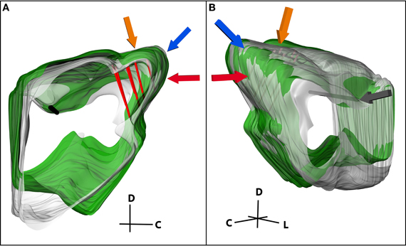
Figure 7. (A) Medial and (B) lateral views of two midbrains (green and gray) normalized to each other. The consistent reference track is shown in black and three pairs of electrode tracks in red. Three of the landmarks used to normalize the midbrains are highlighted, including the caudal-dorsal surface of the inferior colliculus (IC; blue arrow), the curvature of the IC extending from the dorsal to the lateral surface (orange arrow), and the caudal surface of the IC (red arrow). The midbrains were anchored together on the lateral edge of the consistent reference track (gray arrow) and rotated and scaled relative to that point until the new midbrain (green) was normalized to the standard midbrain (gray). C, caudal; D, dorsal; L, lateral.

Correlating Location with Function

A key advantage of this reconstruction method is the ability to correlate functional neural activity with several anatomical locations for extensive mapping studies across animals. In this study, the spatial organization of three general frequency laminae within the central nucleus of the IC (ICC) across animals was reconstructed from the neurophysiological and anatomical data. In vivo experiments were conducted within a sound attenuating, electrically-shielded room, and controlled by a computer using TDT hardware (Tucker-Davis Technology, Alachua, FL) and custom software written in MATLAB (MathWorks, Natick, MA). The TDT-MATLAB system digitally generates acoustic stimuli at a 200 kHz D/A sampling rate (24 bit sigma-delta). Acoustic stimulation was presented via a speaker coupled with the left ear canal by a custom-made hollow ear bar. The speaker-ear bar system was calibrated by coupling the tip of the ear bar with a 0.25-in ACO Pacific condenser microphone (Belmont, CA) via a short plastic tube that represents the ear canal. The neural data was sampled at a rate of 25 kHz (16-bit), passed through analog DC-blocking and anti-aliasing filters up to 7.5 kHz, and later digitally filtered between 0.3 and 3 kHz for spike analysis.

Neural activity was recorded in response to 100 trials of 70 dB SPL, 50 ms duration (0.5 ms rise/fall ramp times) broadband noise (6 octaves centered at 5 kHz) and post-stimulus time histograms were plotted for visualization. Additionally, frequency response maps were plotted by varying 50 ms (5 ms rise/fall ramp times) pure tones (1–40 kHz in 8 steps/octave) from 0 to 70 dB SPL and recording the normalized spike rates for four trials of each stimulus (Figure 8). The spike rate was calculated by finding when the voltage exceeded 3.5 standard deviations above the noise floor within a window of 5–65 ms following the onset of the acoustic stimulus. The best frequency (BF) of each electrode site was determined by taking the centroid of activity across frequencies at 10 dB above the visually-identified threshold level. This BF measure was used instead of characteristic frequency (i.e., frequency corresponding to the maximum activity at threshold) because it was less susceptible to noise and more consistent with what was visually estimated from the frequency response maps.

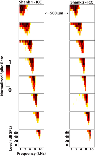
Figure 8. Frequency response maps for two electrode shanks separated by 500 μm placed in the central nucleus of the inferior colliculus (ICC). ICC placements are characterized by sharp tuning and a consistent tonotopic shift from low (superficial sites) to high (deep sites) frequencies. Spike rates were normalized to the maximum number of spikes for each site across all stimuli. Every other site (200 μm spacing) along the electrode shank is plotted. The colorbar was adjusted to remove spontaneous activity to enhance visualization of the response maps.

Results

The first validation of our method was to qualitatively compare our computer model (Figures 3E and F) of the midbrain to images of the midbrain taken a day before slicing. Overlaying our reconstruction on the fixed midbrain (dorsal view shown in Figures 3A and B and lateral view in Figures 3C and D) shows a close correspondence in shape and size of the midbrain. We also quantified the errors associated with the reconstruction process, starting with the accuracy of aligning slices. Another major source of error is due to the subjectivity involved with tracing and aligning the different slices together. Four trained individuals independently reconstructed the same midbrain and we calculated the variation in electrode and reference track locations across slices and for a fully reconstructed midbrain. When normalizing across different midbrains, there is the additional variation of midbrain size and shape that cannot be avoided. Even with this animal variation, we were able to consistently reconstruct several frequency laminae of the ICC across three different animals.

Alignment Error: Analysis of Electrode Shank Best Fit Lines

The accuracy of aligning slices throughout a brain was determined by analyzing the variability in electrode shank points from the best fit line placed through them. Sources of error include tissue deformation while slicing and mounting the sections on slides and manually determining electrode shank locations. Twelve total electrode shanks were randomly chosen from three brains for the analysis. For each electrode shank location within a slice, a perpendicular line was drawn from the placement to the best fit line and measured. Across all of the placements, we found an average distance of 31 μm (standard deviation (σ) = 21 μm, maximum = 260 μm). A distribution of the measured distances (Figure 9) encouragingly shows that ~75% of the electrode shank locations are within 50 μm of their best fit line.

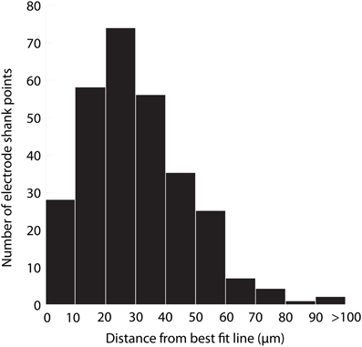
Figure 9. Histogram of the distance of electrode shank points from their best fit line. Twelve total electrode shanks were randomly chosen from three brains. For each electrode shank, a perpendicular line was drawn between the electrode shank location (i.e., point) in each slice and the best fit line across slices. The distance of this perpendicular line was measured across slices, shanks and animals, and the values are displayed in the histogram, which presents the accuracy of alignment across slices. N = 290 electrode shank points.

Single Slice Error: Selection of Electrode and Reference Points

The second analysis performed was to quantify the error of different individuals reconstructing slices and choosing the locations of electrode and reference points (Figure 10). Variations in measurements arise from several sources. For example, the Di-I diffuses through the tissue and the trained individual has to estimate the center of the electrode or reference point. Additionally, the reference needle can cause tearing in the surrounding tissue requiring subjective estimation of the center of the reference point. In order to quantify the individual variation, four individuals reconstructed the same five slices of a midbrain independently. Each slice consisted of three placements of the bi-shank electrode (for a total of six electrode points) and three reference points. The tracings for each slice were then superimposed directly on top of each other by aligning the frame used in Rhinoceros for tracing the slices and the distance between corresponding points across the four individuals were measured. The electrode placements were found to have an average distance of 12 μm (σ = 9 μm, maximum = 61 μm) across all the points and slices. As expected, the reference points had a larger average error of 18 μm (σ = 13 μm, maximum = 61 μm). Consistent localization of reference points is especially important as all of the slices are aligned according to these three points.

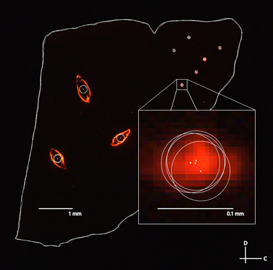
Figure 10. A fluorescent image of a sagittal slice traced by four separate individuals for the second error analysis. The large white circles correspond to the three reference points and the small white circles correspond to the different electrode track placements (three bi-shank placements). Tracing error between individuals was determined by measuring the distance between the estimated electrode track point or reference point (i.e., the center of the circles indicated by white dots) between each pair of individuals, and averaging across all pairs of individuals and placements for five different slices. C, caudal; D, dorsal.

Single Midbrain Error: Identifying Electrode Tracks

While the second analysis provides the individual error associated with simply tracing the slices and selecting points of interest, the next step was to analyze the error associated with the entire three-dimensional reconstruction process, including differences between individuals and the subjective normalization process (Figure 11). Four individuals independently reconstructed the same midbrain. The midbrains were then normalized together as described in the Methods and shown in Figure 8, and five random slices each with six electrode track points (taken from the best fit lines for each electrode shank) were used for analysis. Using this technique and measuring the absolute distances between points for each track across individuals for the different electrode tracks and slices, the average electrode track error was 64 μm (σ = 43 μm, maximum = 201 μm; Figure 11i), which is an error of ~1.5% relative to the entire IC structure (4–5 mm diameter sphere). Since the true electrode track location is likely somewhere between the points estimated by each individual, we performed another analysis that would more closely depict the error of our reconstruction method (Figure 11ii). We calculated the average of the four individuals' best fit lines and assumed this was the actual electrode location for each track (white circle in Figure 11ii). Measuring the distance of each individual's electrode position to this averaged placement across electrode tracks and slices, we found an average error of 31 μm (σ = 19 μm, maximum = 84 μm), corresponding to ~0.7% of the IC structure.

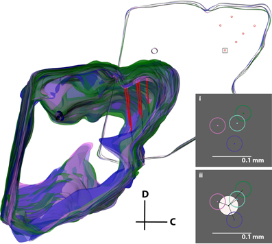
Figure 11. Error analysis procedure incorporating all errors in the reconstruction process. The same midbrain was reconstructed by four different individuals (purple, pink, cyan, and green), aligned, and normalized to each other. The consistent reference track for each midbrain and three pairs of electrode tracks from one of the four midbrains (red) are displayed. A single slice was removed for analysis (top right), and a box around one electrode placement is shown in inserts (i) and (ii). The error was either calculated (i) by taking the distance between each of the four electrode track points (center-to-center of the circles), or (ii) by finding the average of the four placements (white circle) and calculating the distance from its center to each electrode track point. The distances for each of the six electrode points across five slices were averaged to obtain the total error for this analysis. C, caudal; D, dorsal.

Normalizing Across Midbrains: Isofrequency Laminae Analysis

The final analysis sought to qualitatively determine whether our anatomical modeling method could reconstruct electrode site locations across three animals by aligning the neurophysiologically confirmed frequency layers of the ICC (Figure 12). This analysis incorporates both reconstruction errors and inter-animal variability. Based on the literature, layered isofrequency laminae in the ICC are generally accepted to be consistent across animals (Malmierca et al., 1995, 2008; Ehret, 1997; Schreiner and Langner, 1997; Oliver, 2005); thus we expected to see aligned frequency layers across the three animals assuming sufficient accuracy with our reconstruction method. Each midbrain was reconstructed by the same individual and the locations of the isofrequency laminae were determined using in vivo recordings. Isofrequency laminae 0.6 octaves thick, likely corresponding to two critical bands (Schreiner and Langner, 1997; Egorova et al., 2006; Malmierca et al., 2008), were determined. We used 0.6 octaves to have a sufficient number of points per lamina for reconstruction of the layers and because it was not possible with our current method to spatially resolve individual laminae. Electrode site locations with BFs within three ranges—low (2–3.2 kHz), middle (5–8 kHz), and high (10–16 kHz) frequencies—were identified across the three animals and normalized to each other as shown in Figure 12 using the standard midbrain. Encouragingly, the site locations for each lamina aligned consistently across animals and the planes displayed the characteristic ~45° angle (Figure 12B, coronal view).

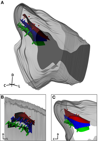
Figure 12. Isofrequency laminae from three midbrains that were aligned and normalized together and shown within the standard midbrain in an isometric view (A), and magnified in a caudal (coronal; B) and lateral (sagittal; C) view. Dots correspond to individual electrode sites with best frequencies measured in vivo via frequency response maps. The curved planes were created in Rhinoceros as a best-fit to the electrode sites. The red, blue, and green planes correspond to low frequency (2–3.2 kHz; n = 26), middle frequency (5–8 kHz, n = 72), and high frequency (10–16 kHz, n = 80) sites, respectively. C, caudal; D, dorsal; L, lateral.

Ideally, these reconstructions can achieve accurate localization of the electrode track and site placements within and across animals. However, due to animal variability, distortions in midbrain shape due to the fixation and reconstruction process, and reconstruction subjectivity, there will always exist some errors that cannot be avoided. Also, this method does not yet possess the resolution to differentiate neighboring isofrequency laminae within the ICC. By using an array with closer sites and improving the reconstruction steps, it will be possible to increase the spatial resolution of the reconstructions. However, as shown in Figure 12, we were still able to differentiate isofrequency laminae separated by 1–2 octaves and map out locations across the ICC laminae. This is useful for studies investigating how coding properties vary within different subregions along the ICC laminae. Although our approach is not yet able to characterize the organization along a single, specific lamina, close-by laminae will likely exhibit similar properties and dimensions, and can be pooled together into one general lamina (Malmierca et al., 1995; Oliver, 2005; Seshagiri and Delgutte, 2007). For example, the low frequency laminae could have different shapes and dimensions than the high frequency laminae (Malmierca et al., 1995). Functional properties as well as afferent and efferent projections can also vary differently between low and high frequency ICC laminae (Ramachandran et al., 1999; Cant and Benson, 2003; Loftus et al., 2004; McMullen et al., 2005). Therefore, separating the ICC into several frequency groups that each may span several critical bands and reconstructing the functional properties and projection pathways along those grouped ICC laminae would provide important and useful information for central auditory processing and organization. Encouragingly, our lab has already identified the existence of functional subregions across and along the ICC laminae using many of the reconstruction steps presented in this paper. This includes both ascending and descending functional and anatomical patterns (Lim and Anderson, 2007a,b; Neuheiser et al., 2010; Markovitz and Lim, 2012).

Discussion

In this study we presented a relatively easy and consistent approach for creating three-dimensional reconstructions of electrode tracks within the IC as well as identifying BF laminae using functional data obtained via electrode sites along those tracks. While electrode locations cannot be perfectly determined due to processing errors, subjectivity within the method and variability between animals, general functional trends can be correlated with anatomical locations using this process. The reconstruction process requires a significant time commitment for tracing and aligning of the slices. However, since the method can be quickly learned, it can serve as a starting project for undergraduate students and even high schools students interested in obtaining initial exposure to neurophysiological and anatomical studies. Automating the different reconstruction steps has been attempted with varying degrees of success by other groups (Ju et al., 2006; Dauguet et al., 2007; Chklovskii et al., 2010; Cifor et al., 2011; Kleinfeld et al., 2011), but these algorithms may miss tissue abnormalities that can generally be fixed through visual and manual correction of the imaged tissue. The customized software packages and additional equipment required for automatic and semi-automatic reconstruction steps can also be quite expensive and not readily available to most neurophysiology labs. For example, four commonly used software packages, Neurolucida (MBF Bioscience, Williston, VT), Amira (Visage Imaging, Richmond VIC, Australia), Avizo (Visualization Science Group, Burlington, MA), and Analyze (AnalyzeDirect, Overland Park, KS), cost between $4000 and $6500 per license, which can become quite expensive when multiple licenses are required. As long as the software is low in cost and multiple licenses and computers can be purchased (e.g., we have four workstations for <$1500 each), a volunteer student infrastructure can provide sufficient personnel time to carefully assess the tissue slices and perform reliable reconstructions, making it more feasible to implement for typical neurophysiological labs. Other costs involved with the procedure can also be minimized, such as by preparing histological slices within the lab instead of outsourcing them to a histology center. While the training and equipment costs are greater initially, this approach is financially beneficial and ensures consistency in the long run.

While this study focused on reconstructing the guinea pig IC using sagittal slices, the process can be utilized across multiple brain regions, species, and slicing planes. One of the most crucial steps in this process is to identify consistent landmarks for normalizing across animals, which would need to be developed for the region of interest. The intersection of the SC, thalamus, and lateral extension from the IC (black arrow in Figure 3C) was used as the consistent landmark for IC reconstructions in guinea pigs. This landmark can be used regardless of the slicing plane, as long as additional reference tracks are made perpendicular to the slicing plane to initially align the slices. The consistent reference track can then be reconstructed and anchored at its lateral-most point for normalization. This landmark can also be used to reconstruct other surrounding and connected brain regions, such as the SC, various thalamic areas, and other brainstem regions. Reconstruction of cortical regions, such as the auditory cortex, may be possible by using the indentation along the pseudosylvian sulcus combined with the edges of the visual, temporal, and frontal cortices and the midline for normalization (cortex is shown in Figures 2A and B). However, since cortical regions are more easily warped during the histology process, other steps such as embedding the tissue in albumin-gelatin or paraffin wax, or slicing on a cryostat may be necessary for increased accuracy (see below for additional improvements).

There are still several hurdles that need to be overcome to create a standard reconstruction method that can be reliably used across research groups. A non-trivial issue with combining data across multiple labs using different software systems is the compatibility of data files. One of the formats that can be used in the Rhinoceros program is AutoCAD.dxf, which is compatible with files produced in Neurolucida, Amira, Avizo, and Analyze. In addition, Rhinoceros files can be saved in over 30 different file formats, allowing for easy manipulation of the data and the potential to fuse files developed from different software programs and research groups. Another issue with combining data across research groups is ensuring that similar fixation and slicing protocols are used to minimize size and shape variations that can affect the reconstructions (Bohland et al., 2009). Transcardial perfusion would improve reconstructions, and should be used for histological protocols to analyze cellular morphology and function. In our study, we did not perform transcardial perfusion since the various experiments in our laboratory typically last 15–20 h and it is not uncommon for the animal to die from the anesthesia before euthanization, preventing successful perfusion of the tissue. However, perfusion can be employed in place of our simple fixation method without changing the rest of the procedure. Even with transcardial perfusion, tissue deformations and shape changes can occur throughout several steps of the reconstruction process (Dauguet et al., 2007). There are global deformations and shrinkage caused by extraction of the brain from the skull and the fixation process as well as loss of cerebrospinal fluid and dehydration. There are also additional local deformations caused by the slicing, mounting of tissue onto the slides, and any additional staining or manipulations of the slices. As further discussed below, MRI reconstructions can be used to identify and address the global deformations, though this approach is not readily available to all labs and can be expensive for a large number of brain reconstructions. One solution is to embed the tissue in a gelatin albumin to prevent deformations cased by mounting the tissue. Another solution is to take images of the blocked tissue surface (i.e., blockface photograph) after each slice of tissue is removed (Dauguet et al., 2007; Bohland et al., 2009). Then the image of the slice mounted onto the slide can be adjusted using various software algorithms to match the blockface photograph. It is possible to also perform three-dimensional reconstruction of the blockface photographs with greater accuracy than with the histological slices. However, the fine anatomical features cannot be clearly identified without the use of appropriate stains that are possible with the histological slices. For our track reconstructions, it was not possible to consistently detect and reconstruct the red-stained track trajectories in blockface photographs. Attempting to create a green filter microscope system combined with the microtome device for capturing both fluorescence and blockface photographs is not trivial and can be expensive. At this stage, it is more realistic to use the blockface photographs to fix the local deformations in the slices, and then use those imaged histological slices for the actual reconstruction process.

Another major hurdle is how to address animal variability, especially when attempting to normalize brains across different animal strains and ages. The normalization process depends on the consistency of anatomical landmarks and edge shapes across animals. For this study, we used guinea pigs that were the same strain and similar in age and weight. Based on visual inspection, we generally observed consistent brain shapes and landmarks across animals, though there were slight variations as observed in Figure 7. One approach to assess how much of these differences are due to the fixation and reconstruction process versus true animal variability is to use MRI to image the in vivo brains of the animals with high spatial resolution (Dauguet et al., 2007). While MRI images could provide confirmation of the histological brain reconstruction method and its consistency across different strains and ages, MRI facilities are not accessible to all neurophysiology labs. Also, morphological and neurochemical assessment of the tissue on the cellular level would not be possible with MRI alone. If MRI facilities and resources are readily available with reduced costs, then it could be possible to complement the histological reconstructions with MRI images. In terms of reconstruction of actual electrode locations throughout the target structure, it may be possible to induce electrolytic lesions large enough to be detected in the MRI images. In our study, we did not use lesions to mark the electrode locations to avoid excessive damage to the tissue, especially since several array placements were made during the experiment. Developing methods for marking the actual electrode locations in vivo without further compromising the neural tissue or functional responses will provide improvements for both histological and MRI reconstruction methods.

The results presented in this study, in addition to the financial and personnel infrastructure described above, are encouraging for developing a standard reconstruction approach that can be performed by multiple labs and used to pool data across animals for creating a more detailed three-dimensional functional model of the brain. One possibility is to have different labs provide their brain models online (i.e., as a Rhinoceros or other compatible file), allowing the community access to the data for further interpretation of coding properties. As long as consistent landmarks are used, groups can normalize the downloaded reconstructions to align with their models. This approach can also be used for brain reconstructions and functional mapping in humans. There has been a significant increase in patients being implanted with neural implants in different brain regions (Zhou and Greenbaum, 2009; Lyons, 2011; Tierney et al., 2011). Coupled with these implants is an enormous amount of perceptual data relating to the effects of stimulation of different locations. Initial identification of the electrode locations are currently achieved through non-invasive CT-MRI techniques. However, confirmation of these locations can also be achieved through histological reconstructions of the implanted brains that become available for research purposes. The functional trends found in humans can then be compared with those from animals.

In summary, our described method allows reconstruction of electrode sites at a spatial resolution of about 100 μm. Additional variability across animals and processing deformations limit identification of absolute locations throughout a structure. However, the use of reliable landmarks and proper normalization as described for our method enables consistent identification of electrode locations across animals to observe general spatial trends along a target nucleus. More sophisticated yet accessible methods and technologies will be necessary to achieve more spatially resolved reconstructions, especially at the cellular and synaptic levels (Bohland et al., 2009; Kleinfeld et al., 2011), and for pooling these data across studies and research groups. Clinically, better understanding of function versus location will help guide optimal electrode placements for neural prosthetic applications and brain-machine devices.

Conflict of Interest Statement

The authors declare that the research was conducted in the absence of any commercial or financial relationships that could be construed as a potential conflict of interest.

Acknowledgments

The authors would like to thank Jessica Pohl, Kyle Wesen, and Patrick Hogan for performing independent reconstructions of the brains for data analysis and for their assistance in preparing figures for the manuscript as well as Sarah Offutt and Malgorzata Straka for feedback on the reconstruction approach and manuscript. We would also like to thank John Oja for assistance with the fluorescence microscopy and Nell Cant for providing her protocols in preparing the histological slices. This work was supported by NIH NIDCD R03-DC011589, NIH NIDA T32-DA022616, the University of Minnesota Institute for Engineering in Medicine Walter Barnes Lange Memorial Award, and start-up funds from the University of Minnesota (Institute for Translational Neuroscience and College of Science and Engineering).

References

Bamann, C., Nagel, G., and Bamberg, E. (2010). Microbial rhodopsins in the spotlight. Curr. Opin. Neurobiol. 20, 610–616.
Bledsoe, S. C., Shore, S. E., and Guitton, M. J. (2003). Spatial representation of corticofugal input in the inferior colliculus: a multicontact silicon probe approach. Exp. Brain Res. 153, 530–542.
Bohland, J. W., Wu, C., Barbas, H., Bokil, H., Bota, M., Breiter, H. C., Cline, H. T., Doyle, J. C., Freed, P. J., Greenspan, R. J., Haber, S. N., Hawrylycz, M., Herrera, D. G., Hilgetag, C. C., Huang, Z. J., Jones, A., Jones, E. G., Karten, H. J., Kleinfeld, D., Kotter, R., Lester, H. A., Lin, J. M., Mensh, B. D., Mikula, S., Panksepp, J., Price, J. L., Safdieh, J., Saper, C. B., Schiff, N. D., Schmahmann, J. D., Stillman, B. W., Svoboda, K., Swanson, L. W., Toga, A. W., Van Essen, D. C., Watson, J. D., and Mitra, P. P. (2009). A proposal for a coordinated effort for the determination of brainwide neuroanatomical connectivity in model organisms at a mesoscopic scale. PLoS Comput. Biol. 5:e1000334. doi: 10.1371/journal.pcbi.1000334
Cant, N. B., and Benson, C. G. (2003). Parallel auditory pathways: projection patterns of the different neuronal populations in the dorsal and ventral cochlear nuclei. Brain Res. Bull. 60, 457–474.
Cant, N. B., and Benson, C. G. (2005). An atlas of the inferior colliculus of the gerbil in three dimensions. Hear. Res. 206, 12–27.
Chklovskii, D. B., Vitaladevuni, S., and Scheffer, L. K. (2010). Semi-automated reconstruction of neural circuits using electron microscopy. Curr. Opin. Neurobiol. 20, 667–675.
Cifor, A., Bai, L., and Pitiot, A. (2011). Smoothness-guided 3-D reconstruction of 2-D histological images. Neuroimage 56, 197–211.
Dauguet, J., Delzescaux, T., Conde, F., Mangin, J. F., Ayache, N., Hantraye, P., and Frouin, V. (2007). Three-dimensional reconstruction of stained histological slices and 3D non-linear registration with in-vivo MRI for whole baboon brain. J. Neurosci. Methods 164, 191–204.
DiCarlo, J. J., Lane, J. W., Hsiao, S. S., and Johnson, K. O. (1996). Marking microelectrode penetrations with fluorescent dyes. J. Neurosci. Methods 64, 75–81.
Egorova, M., Vartanyan, I., and Ehret, G. (2006). Frequency response areas of mouse inferior colliculus neurons: II. Critical bands. Neuroreport 17, 1783–1786.
Ehret, G. (1997). “The auditory midbrain, a “shunting yard” of acoustical information processing,” in The Central Auditory System, eds G. Ehret and R. Romand (New York, NY: Oxford University Press, Inc.), 259–316.
Falcone, J. D., and Bhatti, P. T. (2011). Current steering and current focusing with a high-density intracochlear electrode array. Conf. Proc. IEEE Eng. Med. Biol. Soc. 2011, 1049–1052.
Fenno, L., Yizhar, O., and Deisseroth, K. (2011). The development and application of optogenetics. Annu. Rev. Neurosci. 34, 389–412.
Glover, G. H. (2011). Overview of functional magnetic resonance imaging. Neurosurg. Clin. N. Am. 22, 133–139, vii.
Hemm, S., and Wardell, K. (2010). Stereotactic implantation of deep brain stimulation electrodes: a review of technical systems, methods and emerging tools. Med. Biol. Eng. Comput. 48, 611–624.
Jain, R., and Shore, S. (2006). External inferior colliculus integrates trigeminal and acoustic information: unit responses to trigeminal nucleus and acoustic stimulation in the guinea pig. Neurosci. Lett. 395, 71–75.
Johnson, M. D., Miocinovic, S., McIntyre, C. C., and Vitek, J. L. (2008). Mechanisms and targets of deep brain stimulation in movement disorders. Neurotherapeutics 5, 294–308.
Ju, T., Warren, J., Carson, J., Bello, M., Kakadiaris, I., Chiu, W., Thaller, C., and Eichele, G. (2006). 3D volume reconstruction of a mouse brain from histological sections using warp filtering. J. Neurosci. Methods 156, 84–100.
Kleinfeld, D., Bharioke, A., Blinder, P., Bock, D. D., Briggman, K. L., Chklovskii, D. B., Denk, W., Helmstaedter, M., Kaufhold, J. P., Lee, W. C., Meyer, H. S., Micheva, K. D., Oberlaender, M., Prohaska, S., Reid, R. C., Smith, S. J., Takemura, S., Tsai, P. S., and Sakmann, B. (2011). Large-scale automated histology in the pursuit of connectomes. J. Neurosci. 31, 16125–16138.
Leergaard, T. B., White, N. S., De Crespigny, A., Bolstad, I., D'arceuil, H., Bjaalie, J. G., and Dale, A. M. (2010). Quantitative histological validation of diffusion MRI fiber orientation distributions in the rat brain. PLoS ONE 5:e8595. doi: 10.1371/journal.pone.0008595
Lehew, G., and Nicolelis, M. A. L. (2008). “State-of-the-art microwire array design for chronic neural recordings in behaving animals,” in Methods for Neural Ensemble Recordings, 2nd Edn. ed M. A. L. Nicolelis (Boca Raton, FL), 1–20.
Lenglet, C., Abosch, A., Yacoub, E., De Martino, F., Sapiro, G., and Harel, N. (2012). Comprehensive in vivo mapping of the human basal ganglia and thalamic connectome in individuals using 7T MRI. PLoS ONE 7:e29153. doi: 10.1371/journal.pone.0029153
Lenglet, C., Campbell, J. S., Descoteaux, M., Haro, G., Savadjiev, P., Wassermann, D., Anwander, A., Deriche, R., Pike, G. B., Sapiro, G., Siddiqi, K., and Thompson, P. M. (2009). Mathematical methods for diffusion MRI processing. Neuroimage 45, S111–S122.
Lim, H. H., and Anderson, D. J. (2006). Auditory cortical responses to electrical stimulation of the inferior colliculus: implications for an auditory midbrain implant. J. Neurophysiol. 96, 975–988.
Lim, H. H., and Anderson, D. J. (2007a). Antidromic activation reveals tonotopically organized projections from primary auditory cortex to the central nucleus of the inferior colliculus in guinea pig. J. Neurophysiol. 97, 1413–1427.
Lim, H. H., and Anderson, D. J. (2007b). Spatially distinct functional output regions within the central nucleus of the inferior colliculus: implications for an auditory midbrain implant. J. Neurosci. 27, 8733–8743.
Lim, H. H., Lenarz, M., and Lenarz, T. (2009). Auditory midbrain implant: a review. Trends Amplif. 13, 149–180.
Lim, H. H., Lenarz, M., and Lenarz, T. (2011). “Midbrain auditory prostheses,” in Auditory Prostheses: New Horizons, eds F. G. Zeng, R. R. Fay, and A. N. Popper (New York, NY: Springer Science+Business Media, LLC), 207–232.
Lim, H. H., Lenarz, T., Joseph, G., Battmer, R. D., Samii, A., Samii, M., Patrick, J. F., and Lenarz, M. (2007). Electrical stimulation of the midbrain for hearing restoration: insight into the functional organization of the human central auditory system. J. Neurosci. 27, 13541–13551.
Loftus, W. C., Bishop, D. C., and Oliver, D. L. (2010). Differential patterns of inputs create functional zones in central nucleus of inferior colliculus. J. Neurosci. 30, 13396–13408.
Loftus, W. C., Bishop, D. C., Saint Marie, R. L., and Oliver, D. L. (2004). Organization of binaural excitatory and inhibitory inputs to the inferior colliculus from the superior olive. J. Comp. Neurol. 472, 330–344.
Lozano, A. M., and Hamani, C. (2004). The future of deep brain stimulation. J. Clin. Neurophysiol. 21, 68–69.
Lyons, M. K. (2011). Deep brain stimulation: current and future clinical applications. Mayo Clin. Proc. 86, 662–672.
Malmierca, M. S., Izquierdo, M. A., Cristaudo, S., Hernandez, O., Perez-Gonzalez, D., Covey, E., and Oliver, D. L. (2008). A discontinuous tonotopic organization in the inferior colliculus of the rat. J. Neurosci. 28, 4767–4776.
Malmierca, M. S., Rees, A., Le Beau, F. E., and Bjaalie, J. G. (1995). Laminar organization of frequency-defined local axons within and between the inferior colliculi of the guinea pig. J. Comp. Neurol. 357, 124–144.
Markovitz, C. D., and Lim, H. H. (2012). Dissecting the corticofugal pathways of the central auditory system: the effect of cortical stimulation on neural firing in the inferior colliculus. Assoc. Res. Otolaryngol. Abstr. 35, 274.
McMullen, N. T., Velenovsky, D. S., and Holmes, M. G. (2005). Auditory thalamic organization: cellular slabs, dendritic arbors and tectothalamic axons underlying the frequency map. Neuroscience 136, 927–943.
Merzenich, M. M., and Reid, M. D. (1974). Representation of the cochlea within the inferior colliculus of the cat. Brain Res. 77, 397–415.
Middlebrooks, J. C., and Snyder, R. L. (2007). Auditory prosthesis with a penetrating nerve array. J. Assoc. Res. Otolaryngol. 8, 258–279.
Miesenbock, G. (2011). Optogenetic control of cells and circuits. Annu. Rev. Cell Dev. Biol. 27, 731–758.
Neuheiser, A., Lenarz, M., Reuter, G., Calixto, R., Nolte, I., Lenarz, T., and Lim, H. H. (2010). Effects of pulse phase duration and location of stimulation within the inferior colliculus on auditory cortical evoked potentials in a guinea pig model. J. Assoc. Res. Otolaryngol. 11, 689–708.
Oliver, D. L. (2005). “Neuronal organization in the inferior colliculus,” in The Inferior Colliculus, eds J. A. Winer and C. E. Schreiner (New York, NY: Springer Science+Business Media, Inc.), 69–114.
Ramachandran, R., Davis, K. A., and May, B. J. (1999). Single-unit responses in the inferior colliculus of decerebrate cats. I. Classification based on frequency response maps. J. Neurophysiol. 82, 152–163.
Schreiner, C. E., and Langner, G. (1997). Laminar fine structure of frequency organization in auditory midbrain. Nature 388, 383–386.
Seshagiri, C. V., and Delgutte, B. (2007). Response properties of neighboring neurons in the auditory midbrain for pure-tone stimulation: a tetrode study. J. Neurophysiol. 98, 2058–2073.
Stevenson, I. H., and Kording, K. P. (2011). How advances in neural recording affect data analysis. Nat. Neurosci. 14, 139–142.
Sutton, B. P., Ouyang, C., Karampinos, D. C., and Miller, G. A. (2009). Current trends and challenges in MRI acquisitions to investigate brain function. Int. J. Psychophysiol. 73, 33–42.
Tierney, T. S., Sankar, T., and Lozano, A. M. (2011). Deep brain stimulation emerging indications. Prog. Brain Res. 194, 83–95.
Van Essen, D. C., Ugurbil, K., Auerbach, E., Barch, D., Behrens, T. E., Bucholz, R., Chang, A., Chen, L., Corbetta, M., Curtiss, S. W. Della Penna, S., Feinberg, D., Glasser, M. F., Harel, N., Heath, A. C., Larson-Prior, L., Marcus, D., Michalareas, G., Moeller, S., Oostenveld, R., Petersen, S. E., Prior, F., Schlaggar, B. L., Smith, S. M., Snyder, A. Z., Xu, J., and Yacoub, E. (2012). The Human Connectome Project: a data acquisition perspective. Neuroimage. doi: 10.1016/j.neuroimage.2012.02.018. [Epub ahaed of print].
Yacoub, E., Harel, N., and Ugurbil, K. (2008). High-field fMRI unveils orientation columns in humans. Proc. Natl. Acad. Sci. U.S.A. 105, 10607–10612.
Zhou, D. D., and Greenbaum, E. (eds.). (2009). Implantable Neural Prostheses 1: Devices and Applications. New York, NY: Springer Science+Business Media, LLC.
Zrinzo, L., Yoshida, F., Hariz, M. I., Thornton, J., Foltynie, T., Yousry, T. A., and Limousin, P. (2011). Clinical safety of brain magnetic resonance imaging with implanted deep brain stimulation hardware: large case series and review of the literature. World Neurosurg. 76, 164–172; discussion 169–173.
Keywords: histology, imaging, inferior colliculus, neural prosthesis, deep brain stimulation, population coding, reconstruction, tonotopy
Citation: Markovitz CD, Tang TT, Edge DP and Lim HH (2012) Three-dimensional brain reconstruction of in vivo electrode tracks for neuroscience and neural prosthetic applications. Front. Neural Circuits 6:39. doi: 10.3389/fncir.2012.00039
Received: 06 April 2012; Accepted: 08 June 2012;
Published online: 27 June 2012.
Edited by:
Manuel S. Malmierca, University of Salamanca, SpainReviewed by:
Yang Dan, University of California, USADouglas L. Oliver, University of Connecticut Health Center, USA
Copyright: © 2012 Markovitz, Tang, Edge and Lim. This is an open-access article distributed under the terms of the Creative Commons Attribution Non Commercial License, which permits non-commercial use, distribution, and reproduction in other forums, provided the original authors and source are credited.
*Correspondence: Craig D. Markovitz, Department of Biomedical Engineering, University of Minnesota, 7-105 Hasselmo Hall, 312 Church Street SE, Minneapolis, MN 55455, USA. e-mail: cdmarkovitz@gmail.com
† These authors contributed equally to this work.