

Article Figures & Data
Figures
- Figure 1.
In vivo imaging of visual-evoked responses of layer 2/3 neurons. A, Top, A two-photon image (maximum projection) from L2/3 neurons in mouse primary visual cortex, loaded with OGB-1. Scale bar, 100 μm. B, Example traces of Ca2+ signals from 10 cells during the presentation of drifting gratings with 4 different spatial frequencies and 12 directions. C, Ca2+ responses of two neurons, displayed as a matrix of all stimulus conditions. Columns indicate the direction of motion of the gratings, and rows indicate their SF. Each trial is shown in gray (n = 7); average response across trials of a given stimulus is shown in black. D, Tuning matrix of eight cells (cells 1 and 2 are shown in C). Left, Response matrices evoked by each stimulus. Pixels intensity corresponds to the average ΔF/F over two frames poststimulus presentation and over seven repetitions. Right, Direction–tuning curves fitted with a double Gaussian, measured in various SFs. Colors correspond to SFs marked with arrows next to the matrices on the left.
- Figure 2.
Dependence of orientation tuning curves on SF. A, Comparison of tuning parameters between the preferred SF of each cell and one lower SF. Shown are scatter plots of cells from one network that had preferred SF of ≥0.02 cpd (n = 67 cells). Each circle represents a cell, and the cross represents the population average. Shown from left to right are the ΔF/F to the Pref, ΔF/F to the Orth, OSI, 1-CirVar, HWHH, and the preferred orientation. (Note that the preferred orientation is determined according to the average response across SFs; therefore, a few cells exhibit a marginally higher Pref response to nonoptimal SFs.) B, Comparison of tuning parameters between the preferred SF of each cell and one higher SF. Scatter plots of cells with preferred SF of ≤0.04 cpd (n = 73 cells). Shown are the same parameters as seen in A. C, Histogram of the shift in the preferred orientation with a change in SF. Left, The absolute value of the difference between the lower SF and the preferred SF. Right, The absolute value of the difference between the higher SF and the preferred SF. D, The average shift in the preferred orientation across all the tuned cells (n = 83) aligned according to the preferred SF. E, Population mean showing the change in tuning parameters, pooled from five animals. Gray lines depict individual animals, and black lines depict the mean ± SEM across animals.
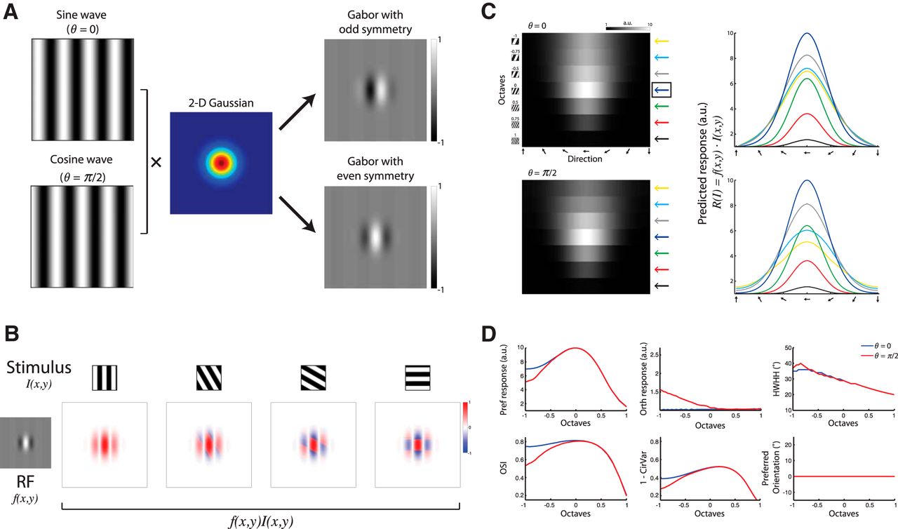
- Figure 3.
Predicting the responses of a simple cell based on an RF model of a 2D symmetric Gabor model. A, A 2D-oriented Gabor function: a sinusoidal plane wave weighted by a Gaussian envelope in two different phases: θ = 0 (sine wave) or θ = π/2 (cosine wave) shown at the top and bottom panels that generate Gabor filters with odd and even symmetry, respectively. B, Constructing spatiotemporally oriented impulse responses from gratings stimuli drifting against a Gabor RF. Top, Examples of stimuli with four different orientations. Bottom, Left, An example of a Gabor RF with θ = π/2. Bottom, Right, Four examples where each box depicts the overlap of the grating stimulus crossing the RF in a phase that yields the maximum response, calculated as the inner product between the stimulus and the RF. C, A predicted response tuning matrix computed as the inner product between the Gabor RF model shown in A, and stimuli of square-wave gratings with various orientations (1º interval) and seven SFs. Each pixel represents the inner product between the RF and the stimulus (maximized across phase, see Materials and Methods). The row marked with a blue arrow on the right denotes the preferred SF and was taken as a reference for comparing other SFs. Right, Orientation tuning curves at various SFs, color coded according to the arrows shown next to the predicted tuning matrix. Top and bottom panels correspond to RF with θ = 0 and θ = π/2, respectively. a.u., Arbitrary units. D, Comparison of orientation tuning parameters between various SFs, based on the predicted response shown in C. Blue and red lines depict the parameters calculated based on a Gabor RF model with θ = 0 and θ = π/2, respectively. Shown are the ΔF/F to the Pref, the ΔF/F to the Orth, OSI, 1 − CirVar, HWHH, and the preferred orientation.
- Figure 4.
Altering the Gabor model parameters for predicting neural responses. A, A predicted response tuning matrix computed as the inner product between the Gabor RF model shown in Figure 3 and stimuli of square-wave gratings with various orientations (1º interval) and seven SFs. Each pixel represents the inner product between the RF and the stimulus (maximized across phase). The row marked with a blue arrow on the right denotes the preferred SF and was taken as a reference for comparing other SFs. Right, Orientation–tuning curves at various SFs, color coded according to the arrows shown next to the predicted tuning matrix. Each panel corresponds to RF with θ = 0, θ = π/6, θ = π/3, and θ = π/2. a.u., Arbitrary units. B, Same as in A only for an RF with θ = π/2 and various spatial aspect ratios (γ). Each panel corresponds to RF with γ = 1, γ = 1.33, γ = 1.5, and γ = 2. Note that these parameter alterations alone could not qualitatively explain a shift in the preferred orientation of the cells at different SFs.
- Figure 5.
Impulse responses from gratings stimuli drifting against a Gabor RF. A, The impulse responses from gratings stimuli drifting against a Gabor RF in various offsets. Top left, A Gabor RF with θ = π/2. In each row, on the left is the stimulus presented with one orientation; on the right are 11 examples where each box depicts the overlap of the grating stimulus crossing the RF in a particular phase. The box marked with a black border is the phase yielding the maximum response. B, Bottom, The predicted response as a function of phase, calculated as the inner product between the RF and the stimulus at each phase. The predicted response per stimulus was then maximized across phase.
- Figure 6.
Predicting the responses of a simple cell based on an RF model of a 2D tilted Gabor. A, A 2D tilted Gabor function: a sinusoidal plane wave weighted by a tilted Gaussian envelope (the Gaussian was rotated against the orientation of the sinusoidal plane wave) in two different phases: θ = 0 (sine wave) or θ = π/2 (cosine wave) shown at the top and bottom panels, respectively. B, Constructing spatiotemporally oriented impulse responses from gratings stimuli drifting against a tilted Gabor RF. Top, Examples of stimuli with four various orientations. Bottom, Left shows an example of a tilted Gabor RF with θ = π/2. On the right, four examples where each box depicts the overlap of the grating stimulus crossing the RF in a phase that yields the maximum response, calculated as the inner product between the stimulus and the RF. C, A predicted response tuning matrix computed as the inner product between the tilted Gabor RF model shown in A, and stimuli of square-wave gratings with various orientations (1º interval) and seven SFs. Each pixel represents the inner product between the RF and the stimulus (maximized across phase). The row marked with a blue arrow on the right denotes the preferred SF and was taken as a reference for comparing other SFs. Right, Orientation tuning curves at various SFs, color coded according to the arrows shown next to the predicted tuning matrix. Top and bottom panels correspond to RF with θ = 0 and θ = π/2, respectively. D, Comparison of orientation–tuning parameters between various SFs, based on the predicted response shown in C. Blue and red lines depict the parameters calculated based on a tilted Gabor RF model with θ = 0 and θ = π/2, respectively. Shown are the ΔF/F to the Pref, the ΔF/F to the Orth, OSI, 1 − CirVar, HWHH, and the preferred orientation.


In this issue


